Videos
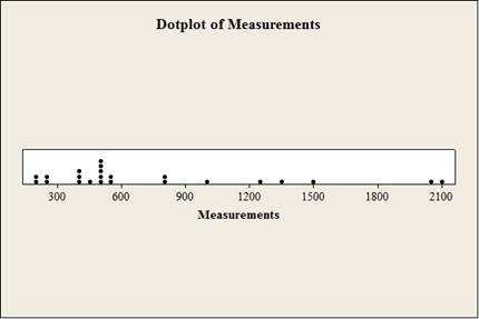
The article “Hydrogeochemical Characteristics of Groundwater in a Mid-Western Coastal Aquifer System” (S. Jeen. J. Kim, et al., Geosciences Journal, 2001:339–348) presents measurements of various properties of shallow groundwater in a certain aquifer system in Korea. Following are measurements of electrical conductivity (in microsiemens per centimeter) for 23 water samples.
2099 528 2030 1350 1018 384 1499
1265 375 424 789 810 522 513
488 200 215 486 257 557 260
461 500
- a. Find the mean.
- b. Find the standard deviation.
- c. Find the median.
- d. Construct a dotplot.
- e. Find the 10% trimmed mean.
- f. Find the first
quartile . - g. Find the third quartile.
- h. Find the
interquartile range . - i. Construct a boxplot.
- j. Which of the points, if any, are outliers?
- k. If a histogram were constructed, would it be skewed to the left, skewed to the right, or approximately symmetric?
a.
Find the mean.
Answer to Problem 16SE
The mean is 740.0.
Explanation of Solution
Given info:
The data shows that the measurements of the electrical conductivity.
Calculation:
Step by step procedure for finding the mean concentration using Minitab software is follows:
- Choose Stat > Basic Statistics > Display Descriptive Statistics.
- In Variables enter the columns Measurements.
- Choose option statistics, and select Mean.
- Click OK.
Output using Minitab software is,
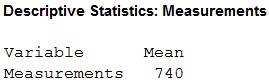
From the output the mean is 74.0.
b.
Find the standard deviation.
Answer to Problem 16SE
The standard deviation is 550.
Explanation of Solution
Calculation:
Step by step procedure for finding the mean concentration using Minitab software is follows:
- Choose Stat > Basic Statistics > Display Descriptive Statistics.
- In Variables enter the columns Measurements.
- Choose option statistics, and select Standard deviation.
- Click OK.
Output using Minitab software is,
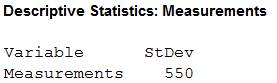
From the output the standard deviation is 550.
c.
Compute the median.
Answer to Problem 16SE
The median is 513.
Explanation of Solution
Calculation:
Step by step procedure for finding the median concentration is follows:
- Choose Stat > Basic Statistics > Display Descriptive Statistics.
- In Variables enter the columns Measurements.
- Choose option statistics, and select Median.
- Click OK.
Output using Minitab software is,
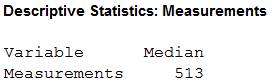
From the output the median is 513.
d.
Construct a dotplot.
Answer to Problem 16SE
The dotplot is,
Explanation of Solution
Calculation:
Step by step procedure to constructing dotplot using Minitab procedure is follows:
- Choose Graph > Dotplot.
- Choose One Y-Simple and then click OK.
- In Graph variables, enter Measurements.
- Click OK.
e.
Compute the 10% trimmed mean.
Answer to Problem 16SE
The 10% trimmed mean is 657.16.
Explanation of Solution
Calculation:
The sample size n is 23.
Trimmed mean:
The trimmed mean is a measure of center that is designed to be unaffected by outliers.
The 10% of the value is,
Therefore, trim the highest 2 and lowest 2 observations from the given data.
The observations after trimmed values are,
| n | Measurements |
| 1 | 257 |
| 2 | 260 |
| 3 | 375 |
| 4 | 384 |
| 5 | 424 |
| 6 | 461 |
| 7 | 486 |
| 8 | 488 |
| 9 | 500 |
| 10 | 513 |
| 11 | 522 |
| 12 | 528 |
| 13 | 557 |
| 14 | 789 |
| 15 | 810 |
| 16 | 1018 |
| 17 | 1265 |
| 18 | 1350 |
| 19 | 1499 |
| Total | 12,486 |
| Mean |
From the table, the trimmed mean is 657.16.
f.
Compute the first quartile.
Answer to Problem 16SE
The first quartile of the concentrations is 384.
Explanation of Solution
Calculation:
Step by step procedure for finding the first quartile of the concentration is follows:
- Choose Stat > Basic Statistics > Display Descriptive Statistics.
- In Variables enter the columns Measurements.
- Choose option statistics, and select First quartile.
- Click OK.
Output using Minitab software is,
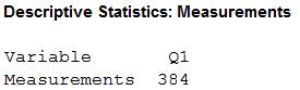
From the output the first quartile is 384.
g.
Compute the third quartile.
Answer to Problem 16SE
The third quartile is 1,018.
Explanation of Solution
Calculation:
Step by step procedure for finding the third quartile of the concentration is follows:
- Choose Stat > Basic Statistics > Display Descriptive Statistics.
- In Variables enter the columns Measurements.
- Choose option statistics, and select Third quartile.
- Click OK.
Output using Minitab software is,
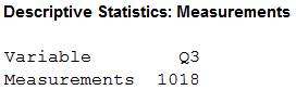
From the output the third quartile is 1,018.
h.
Compute the interquartile range.
Answer to Problem 16SE
The interquartile range is 634.
Explanation of Solution
Calculation:
Step by step procedure for finding the third quartile of the concentration is follows:
- Choose Stat > Basic Statistics > Display Descriptive Statistics.
- In Variables enter the columns Measurements.
- Choose option statistics, and select Interquartile range.
- Click OK.
Output using Minitab software is,
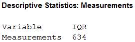
From the output the interquartile range is 634.
i.
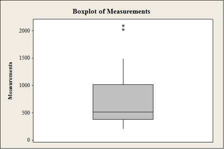
Construct a boxplot for the concentrations.
Answer to Problem 16SE
The boxplot for the given data is,
Explanation of Solution
Calculation:
Step by step procedure to constructing boxplot using Minitab procedure is follows:
- Choose Graph > Boxplot or Stat > EDA > Boxplot.
- Under One Y, choose Simple. Click OK.
- In Graph variables, enter Measurements.
- Click OK.
j.
Identify the points in any outliers.
Answer to Problem 16SE
The points 2,030 and 2,099 are outliers.
Explanation of Solution
Calculation:
Outlier:
If the sample contain a few points that are much larger or smaller than the rest then the points are called outliers.
From the boxplot, it can be concluded that there are two outliers. They are 2,030 and 2,099.
k.
Identify it is skewed to the left, skewed to the right or approximately symmetric if histogram were constructed.
Answer to Problem 16SE
The histogram is skewed to the right.
Explanation of Solution
Calculation:
Left and Right skewed:
If the sample is left skewed then the median is closer to the third quartile than to the first quartile and if the sample is right skewed then the median is closer to the first quartile than to the third quartile.
From the boxplot, it is observed that the median is closer to the first quartile than to the third quartile. That is, the data is skewed to the right.
Therefore, the histogram is skewed to the right.
Want to see more full solutions like this?
Chapter 1 Solutions
Statistics for Engineers and Scientists (Looseleaf)


- The article "Hydrogeochemical Characteristics of Groundwater in a Mid-Western Coastal Aquifer System" (S. Jeen, J. Kim, et al., Geosciences Journal, 2001:339-348) presents measurements of various properties of shallow groundwater in a certain aquifer system in Korea. Following are measurements of electrical conductivity (in microsiemens per centimeter) for 23 water samples. 2099 528 2030 1350 1018 384 1499 1265 375 424 789 810 522 513 488 200 215 486 257 557 260 461 500 a) Find the mean, median, mode, and standard deviation. b) Construct a histogram using relative frequency on the y-axis and comment on the shape of the distribution.arrow_forwardThe article "Hydrogeochemical Characteristics of Groundwater in a Mid-Western Coastal Aquifer System" (S. Jeen, J. Kim, et al., Geosciences Journal, 2001:339–348) presents measurements of various properties of shallow groundwater in a certain aquifer system in Korea. Following are measurements of electrical conductivity (in microsiemens per centimeter) for 23 water samples. 2099 528 2030 1350 1018 384 1499 522 557 1265 375 424 789 810 513 488 200 215 486 257 260 461 500 a. Find the mean. ъ. Find the standard deviation. C. Find the median. d. Construct a dotplot. e. Find the 10% trimmed mean. Find the first quartile. Find the third quartile. Find the interquartile range. Construct a boxplot. f. g- h. i. j. Which of the points, if any, are outliers? k. If a histogram were constructed, would it be skewed to the left, skewed to the right, or approximately symmetric?arrow_forwardThe article "Modeling Resilient Modulus and Temperature Correction for Saudi Roads" (H. Wahhab, I. Asi, and R. Ramadhan, Journal of Materials in Civil Engineering, 2001:298– 305) describes a study designed to predict the resilient modulus of pavement from physical properties. The following table presents data for the resilient modulus at 40°Cin10® kPa (y), the surface area of the aggregate in m²/kg (x1), and the softening point of the asphalt in °C (х). y X1 X2 1.48 5.77 60.5 1.70 7.45 74.2 2.03 8.14 67.6 2.86 8.73 70.0 2.43 7.12 64.6 3.06 6.89 65.3 2.44 8.64 66.2 1.29 6.58 64.1 3.53 9.10 68.6 1.04 8.06 58.8 1.88 5.93 63.2 1.90 8.17 62.1 1.76 9.84 68.9 2.82 7.17 72.2 1.00 7.78 54.1 The full quadratic model is y = + P,x, + PzX, + Pz*jXz + Pxx¡ + Bzx; + €. Which submodel of this full model do you believe is most appropriate? Justify your answer by fitting two or more models and comparing the results.arrow_forward
- The article “Wastewater Treatment Sludge as a Raw Material for the Production of Bacillus thuringiensis Based Biopesticides” (M. Tirado Montiel, R. Tyagi, and J. Valero, Water Research, 2001:3807–3816) presents measurements of total solids, in g/L, for seven sludge specimens. The results (rounded to the nearest gram) are 20, 5, 25, 43, 24, 21, and 32. Assume the distribution of total solids is approximately symmetric. a) Can you conclude that the mean concentration of total solids is greater than 14 g/L? Compute the appropriate test statistic and find the P-value. b) Can you conclude that the mean concentration of total solids is less than 30 g/L? Compute the appropriate test statistic and find the P-value. c) An environmental engineer claims that the mean concentration of total solids is equal to 18 g/L. Can you conclude that the claim is false?arrow_forwardThe depth of wetting of a soil is the depth to which water content will increase owing to extemal factors. The article "Discussion of Method for Evaluation of Depth of Wetting in Residential Areas" (J. Nelson, K. Chao, and D. Overton, Journal of Geotechnical and Geoenvironmental Engineering, 2011:293-296) discusses the relationship between depth of wetting beneath a structure and the age of the structure. The article presents measurements of depth of wetting, in meters, and the ages, in years, of 21 houses, as shown in the following table. Age Depth 7.6 4 4.6 6.1 9.1 3 4.3 7.3 5.2 10.4 15.5 5.8 10.7 4 5.5 6.1 10.7 10.4 4.6 7.0 6.1 14 16.8 10 9.1 8.8 Compute the least-squares line for predicting depth of wetting (y) from age (x). b. Identify a point with an unusually large x-value. Compute the least-squares line that results from deletion of this point. Identify another point which can be classified as an outlier. Compute the least-squares line that results from deletion of the outlier,…arrow_forward7. The article "Hydrogeochemical Characteristics of Groundwater in a Mid-Western Coastal Aquifer System" (S. Jeen, J. Kim, et al., Geosciences Journal, 2001:339-348) presents measurements of various properties of shallow groundwater in a certain aquifer system in Korea. Following are measurements of electrical conductivity (in microsiemens per centimeter) for 23 water samples. 2099 528 2030 1350 1018 384 1499 1265 375 424 789 810 522 513 488 200 215 486 257 557 260 461 500 a. Find the mean. b. Find the standard deviation. c. Find the median. d. Findthe 10%trimmedmean. e. Find the first quartile. f. Find the third quartile. g. Find the interquartile range. h. Construct a boxplot. i. Which of the points, if any, are outliers? j. If a histogram were constructed, would it be skewed to the left, skewed to the right, or approximately symmetric? 8. Forty-five specimens of a certain type of powder were analyzed for sulfur trioxide content. Following are the results, in percent. The list has…arrow_forward
- The article "Characteristics and Trends of River Discharge into Hudson, James, and Ungava Bays, 1964-2000" (S. Dery, M. Stieglitz, et al., Journal of Climate, 2005:2540-2557) presents measurements of discharge rate x (in kmlyr) andpeakflow y (in m/s) for 42 rivers that drain into the Hudson, James, and Ungava Bays. The data are shown in the following table: Discharge Peak Flow 94.24 4110.3 66.57 4961.7 59.79 10275.5 48.52 6616.9 40.00 7459.5 32.30 2784.4 31.20 3266.7 30.69 4368.7 26.65 1328.5 22.75 4437.6 21.20 1983.0 20.57 1320.1 19.77 1735.7 18.62 1944.1 17.96 3420.2 17.84 2655.3 16.06 3470.3 1561.6 14.69 11.63 869.8 11.19 936.8 11.08 1315.7 10.92 1727.1 9.94 768.1 7.86 483.3arrow_forwardFollowing are measurements of soil concentrations (in mg /kg) of chromium (Cr) and nickel (Ni) at20 sites in the area of Cleveland, Ohio. These data are taken from the article "Variation in NorthAmerican Regulatory Guidance for Heavy Metal Surface Soil Contamination at Commercial andIndustrial Sites" (A. Jennings and J. Ma, J. Environment Eng, 2007:587-609). Cr: 260 19 36 247 263 319 317 277 319 264 23 29 61 119 33 281 21 35 64 30Ni: 435 377 359 53 38 38 54 188 397 33 92 490 28 35 799 347 321 32 74 508 (a) Construct a histogram for each set of concentrations. (b) Find the 1st, 2nd and 3rd quartiles for the Cr concentrations (c) Find the 1st, 2nd and 3rd quartiles for the Ni concentrations.arrow_forwardFollowing are measurements of soil concentrations (in mg /kg) of chromium (Cr) and nickel (Ni) at20 sites in the area of Cleveland, Ohio. These data are taken from the article "Variation in NorthAmerican Regulatory Guidance for Heavy Metal Surface Soil Contamination at Commercial andIndustrial Sites" (A. Jennings and J. Ma, J. Environment Eng, 2007:587-609).Cr: 260 19 36 247 263 319 317 277 319 264 23 29 61 119 33 281 21 35 64 30Ni: 435 377 359 53 38 38 54 188 397 33 92 490 28 35 799 347 321 32 74 508 (d) Use these to construct comparative boxplots for the two sets of concentrations. (e) Using the boxplots, what differences can be seen between the two sets of concentrations?arrow_forward
- Fluid inclusions are microscopic volumes of fluid that are trapped in rock during rock formation. The article "Fluid Inclusion Study of Metamorphic Gold-Quartz Veins in Northwestern Nevada, U.S.A.: Characteristics of Tectonically Induced Fluid" (S. Cheong, Geosciences Journal, 2002:103-115) describes the geochemical properties of fluid inclusions in several different veins in northwest Nevada. The following table presents data on the maximum salinity (% NaCi by weight) of inclusions in several rock samples from several areas. Salinity Area Humboldt Range Santa Rosa Range 9.2 10.0 11.2 8.8 5.2 6.1 8.3 Ten Mile 7.9 6.7 9.5 7.3 10.4 7.0 Antelope Range Pine Forest Range 6.7 8.4 9.9 10.5 16.7 17.5 15.3 20.0 Can you conclude that the salinity differs among the areas?arrow_forwardQ3) An experiment was carried out to investigate variation of solubility of chemical X in water. The quantities in kg that dissolved in 1 liter at various temperatures are show in the table (1). Table (1) Temperature C Mass of X 2.1 2.6 2.9 3.3 15 20 25 30 35 4 50 5.1 70 7 Use the proper methods to answer the following questions: a) Draw a scatter diagram to show the data. b) Estimate the temperature based on the mass of X. c) What quantity might be expected to dissolve at 42 C? Find the quantity that your cquation indicates would dissolve at 10 C and comment on your answer.arrow_forwardIn the article “Groundwater Electromagnetic Imaging in Complex Geological and Topographical Regions: A Case Study of a Tectonic Boundary in the French Alps” (S. Houtot, P. Tarits, et al., Geophysics, 2002:1048–1060), the pH was measured for several water samples in various locations near Gittaz Lake in the French Alps. The results for 11 locations on the northern side of the lake and for 6 locations on the southern side are as follows: Northern side: 8.1 8.2 8.1 8.2 8.2 7.4 7.3 7.4 8.1 8.1 7.9 Southern side: 7.8 8.2 7.9 7.9 8.1 8.1 Find a 98% confidence interval for the difference in pH between the northern and southern side.arrow_forward
 MATLAB: An Introduction with ApplicationsStatisticsISBN:9781119256830Author:Amos GilatPublisher:John Wiley & Sons Inc
 Probability and Statistics for Engineering and th...StatisticsISBN:9781305251809Author:Jay L. DevorePublisher:Cengage Learning
 Statistics for The Behavioral Sciences (MindTap C...StatisticsISBN:9781305504912Author:Frederick J Gravetter, Larry B. WallnauPublisher:Cengage Learning
 Elementary Statistics: Picturing the World (7th E...StatisticsISBN:9780134683416Author:Ron Larson, Betsy FarberPublisher:PEARSON
 The Basic Practice of StatisticsStatisticsISBN:9781319042578Author:David S. Moore, William I. Notz, Michael A. FlignerPublisher:W. H. Freeman
 Introduction to the Practice of StatisticsStatisticsISBN:9781319013387Author:David S. Moore, George P. McCabe, Bruce A. CraigPublisher:W. H. Freeman