
Finite Mathematics and Applied Calculus (MindTap Course List)
7th Edition
ISBN: 9781337274203
Author: Stefan Waner, Steven Costenoble
Publisher: Cengage Learning
expand_more
expand_more
format_list_bulleted
Videos
Question
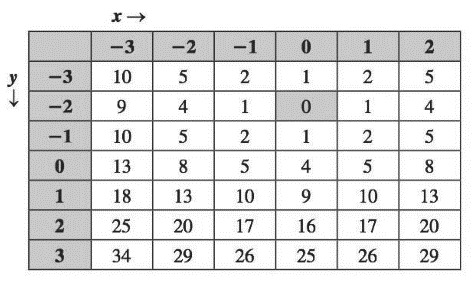
Chapter 15.3, Problem 5E
To determine
The classification of shaded value in the table as one of the following:
Expert Solution & Answer
Want to see the full answer?
Check out a sample textbook solution
Students have asked these similar questions
(a) Determine the maximum and minimum values for each variable in the table
(b) Use your results from part (a) to find an appropriate viewing rectangle
(c) Make a scatterplot of the data
(d) Make a line graph of the data
x(year) 1984|1985 1986 1987 1988 1989
y (sales)13 2.1 3.34.8 5.2 5.5
wnat are tne maximum ana minimum vaiues OT V
y-min1.3 and y-max- 5.5
(b) Choose an appropriate viewing window
yA. [1984,1989,1] by [1,6,0.2]
B. [1,6,0.2] by [1989,1994,1]
O C. [1,6,0.2] by [1984,1989,1]
D. [1989,1994,1] by [1,6,0.2]
(c) Use the viewing rectangle [1980,1995,1] by [1,6,0.2]. Choose the correct scatterplot.
Click to select your answer and then click Check Answer.
The data below are the temperatures on randomly chosen days during the summer and the number of employee absences at a local company on those days. Test the claim, at the α = 0.05 level of significance, that a linear relation exists between the two variables, Apply classical and traditional approaches. Show step1-step3.
Thirty data points on Y and X are employed to estimate the parameters in the linear
relation
Y = a + bx.
The computer output from the regression analysis is
DEPENDENT
VARIABLE:
R-SQUARE
F-RATIO
P-VALUE ON F
OBSERVATIONS:
30
0.5300
13.79
0.0009
VARIABLE
PARAMETER
STANDARD
T-RATIO
P-VALUE
ESTIMATE
ERROR
INTERCEPT
93.54
46.210
2.02
0.0526
|-3.25
0.875
|-3.71
0.0009
At the 1% level of significance, the critical t-value for the test is
(Write the numbers as they are, do not round them)
Chapter 15 Solutions
Finite Mathematics and Applied Calculus (MindTap Course List)
Ch. 15.1 - For each function in Exercises 14, evaluate (a)...Ch. 15.1 - Prob. 2ECh. 15.1 - Prob. 3ECh. 15.1 - Prob. 4ECh. 15.1 - Prob. 5ECh. 15.1 - Prob. 6ECh. 15.1 - Prob. 7ECh. 15.1 - Prob. 8ECh. 15.1 - Prob. 9ECh. 15.1 - Prob. 10E
Ch. 15.1 - Prob. 11ECh. 15.1 - Prob. 12ECh. 15.1 - Prob. 13ECh. 15.1 - Prob. 14ECh. 15.1 - Prob. 15ECh. 15.1 - Prob. 16ECh. 15.1 - Prob. 17ECh. 15.1 - Prob. 18ECh. 15.1 - Prob. 19ECh. 15.1 - Prob. 20ECh. 15.1 - Prob. 21ECh. 15.1 - Prob. 22ECh. 15.1 - The following statistical table lists some values...Ch. 15.1 - Prob. 24ECh. 15.1 - Prob. 25ECh. 15.1 - Prob. 26ECh. 15.1 - Prob. 27ECh. 15.1 - Prob. 28ECh. 15.1 - Prob. 29ECh. 15.1 - Prob. 30ECh. 15.1 - Prob. 31ECh. 15.1 - Prob. 32ECh. 15.1 - Prob. 33ECh. 15.1 - Prob. 34ECh. 15.1 - Prob. 35ECh. 15.1 - Prob. 36ECh. 15.1 - Prob. 37ECh. 15.1 - Prob. 38ECh. 15.1 - Prob. 39ECh. 15.1 - Prob. 40ECh. 15.1 - Prob. 41ECh. 15.1 - Prob. 42ECh. 15.1 - Prob. 43ECh. 15.1 - Prob. 44ECh. 15.1 - Prob. 45ECh. 15.1 - Prob. 46ECh. 15.1 - Prob. 47ECh. 15.1 - Prob. 48ECh. 15.1 - Prob. 49ECh. 15.1 - Prob. 50ECh. 15.1 - Prob. 51ECh. 15.1 - Prob. 52ECh. 15.1 - Prob. 53ECh. 15.1 - Prob. 54ECh. 15.1 - Exercises 55-58 refer to the following plot of...Ch. 15.1 - Prob. 56ECh. 15.1 - Prob. 57ECh. 15.1 - Exercises 55-58 refer to the following plot of...Ch. 15.1 - Prob. 59ECh. 15.1 - Prob. 60ECh. 15.1 - Prob. 61ECh. 15.1 - Prob. 62ECh. 15.1 - Prob. 63ECh. 15.1 - Prob. 64ECh. 15.1 - Prob. 65ECh. 15.1 - Prob. 66ECh. 15.1 - Prob. 67ECh. 15.1 - Prob. 68ECh. 15.1 - Prob. 69ECh. 15.1 - Prob. 70ECh. 15.1 - Prob. 71ECh. 15.1 - Prob. 72ECh. 15.1 - Prob. 73ECh. 15.1 - Prob. 74ECh. 15.1 - Prob. 75ECh. 15.1 - Prob. 76ECh. 15.1 - Prob. 77ECh. 15.1 - Prob. 78ECh. 15.1 - Prob. 79ECh. 15.1 - Scientific Research The number z of research...Ch. 15.1 - Prob. 81ECh. 15.1 - Prob. 82ECh. 15.1 - Prob. 83ECh. 15.1 - Prob. 84ECh. 15.1 - Prob. 85ECh. 15.1 - Prob. 86ECh. 15.1 - Prob. 87ECh. 15.1 - Prob. 88ECh. 15.1 - Prob. 89ECh. 15.1 - Prob. 90ECh. 15.1 - Prob. 91ECh. 15.1 - Housing Costs10? The cost C (in dollars) of...Ch. 15.1 - Prob. 93ECh. 15.1 - Prob. 94ECh. 15.1 - Prob. 95ECh. 15.1 - Prob. 96ECh. 15.1 - Prob. 97ECh. 15.1 - Prob. 98ECh. 15.1 - Prob. 99ECh. 15.1 - Prob. 100ECh. 15.1 - Prob. 102ECh. 15.1 - Prob. 103ECh. 15.1 - Prob. 104ECh. 15.1 - Prob. 105ECh. 15.1 - Prob. 106ECh. 15.1 - Prob. 107ECh. 15.1 - Prob. 108ECh. 15.1 - Prob. 109ECh. 15.1 - Prob. 110ECh. 15.1 - Prob. 111ECh. 15.1 - Prob. 112ECh. 15.1 - Prob. 113ECh. 15.1 - Prob. 114ECh. 15.1 - Prob. 115ECh. 15.1 - Prob. 116ECh. 15.1 - Prob. 117ECh. 15.1 - Prob. 118ECh. 15.1 - Prob. 119ECh. 15.1 - Prob. 120ECh. 15.1 - Prob. 121ECh. 15.1 - Prob. 122ECh. 15.1 - Prob. 123ECh. 15.1 - Prob. 124ECh. 15.2 - Prob. 1ECh. 15.2 - Prob. 2ECh. 15.2 - Prob. 3ECh. 15.2 - Prob. 4ECh. 15.2 - In Exercises 1-18, calculate fx,fy,fx|(1,1), and...Ch. 15.2 - Prob. 6ECh. 15.2 - Prob. 7ECh. 15.2 - Prob. 8ECh. 15.2 - Prob. 9ECh. 15.2 - Prob. 10ECh. 15.2 - Prob. 11ECh. 15.2 - Prob. 12ECh. 15.2 - Prob. 13ECh. 15.2 - Prob. 14ECh. 15.2 - Prob. 15ECh. 15.2 - Prob. 16ECh. 15.2 - Prob. 17ECh. 15.2 - Prob. 18ECh. 15.2 - Prob. 19ECh. 15.2 - Prob. 20ECh. 15.2 - Prob. 21ECh. 15.2 - Prob. 22ECh. 15.2 - Prob. 23ECh. 15.2 - Prob. 24ECh. 15.2 - Prob. 25ECh. 15.2 - Prob. 26ECh. 15.2 - Prob. 27ECh. 15.2 - Prob. 28ECh. 15.2 - Prob. 29ECh. 15.2 - Prob. 30ECh. 15.2 - Prob. 31ECh. 15.2 - Prob. 32ECh. 15.2 - Prob. 33ECh. 15.2 - Prob. 34ECh. 15.2 - Prob. 35ECh. 15.2 - Prob. 36ECh. 15.2 - Prob. 37ECh. 15.2 - Prob. 38ECh. 15.2 - Prob. 39ECh. 15.2 - Prob. 40ECh. 15.2 - Prob. 41ECh. 15.2 - Prob. 42ECh. 15.2 - Prob. 43ECh. 15.2 - Prob. 44ECh. 15.2 - Prob. 45ECh. 15.2 - Marginal Cost (Interaction Model) Your weekly cost...Ch. 15.2 - Prob. 47ECh. 15.2 - Prob. 48ECh. 15.2 - Marginal Cost Your weekly cost (in dollars) to...Ch. 15.2 - Marginal Cost Your weekly cost (in dollars) 10...Ch. 15.2 - Prob. 51ECh. 15.2 - Prob. 52ECh. 15.2 - Prob. 53ECh. 15.2 - Prob. 54ECh. 15.2 - Prob. 55ECh. 15.2 - Prob. 56ECh. 15.2 - Prob. 57ECh. 15.2 - Prob. 58ECh. 15.2 - Prob. 59ECh. 15.2 - Prob. 60ECh. 15.2 - Prob. 61ECh. 15.2 - Prob. 62ECh. 15.2 - Prob. 63ECh. 15.2 - Investments Repeat Exercise 63, using the formula...Ch. 15.2 - Prob. 65ECh. 15.2 - Prob. 66ECh. 15.2 - Prob. 67ECh. 15.2 - Prob. 68ECh. 15.2 - Prob. 69ECh. 15.2 - Prob. 70ECh. 15.2 - Prob. 71ECh. 15.2 - Prob. 72ECh. 15.2 - Prob. 73ECh. 15.2 - Prob. 74ECh. 15.2 - Prob. 75ECh. 15.2 - Prob. 76ECh. 15.3 - In Exercises 1-4, classify each labeled point on...Ch. 15.3 - Prob. 2ECh. 15.3 - Prob. 3ECh. 15.3 - Prob. 4ECh. 15.3 - Prob. 5ECh. 15.3 - Prob. 6ECh. 15.3 - Prob. 7ECh. 15.3 - Prob. 8ECh. 15.3 - Prob. 9ECh. 15.3 - Prob. 10ECh. 15.3 - Prob. 11ECh. 15.3 - Prob. 12ECh. 15.3 - Prob. 13ECh. 15.3 - Prob. 14ECh. 15.3 - Prob. 15ECh. 15.3 - Prob. 16ECh. 15.3 - Prob. 17ECh. 15.3 - Prob. 18ECh. 15.3 - Prob. 19ECh. 15.3 - Prob. 20ECh. 15.3 - Prob. 21ECh. 15.3 - Prob. 22ECh. 15.3 - Prob. 23ECh. 15.3 - Prob. 24ECh. 15.3 - Prob. 25ECh. 15.3 - Prob. 26ECh. 15.3 - Prob. 27ECh. 15.3 - In Exercises 11-36, locate and classify all the...Ch. 15.3 - Prob. 29ECh. 15.3 - Prob. 30ECh. 15.3 - Prob. 31ECh. 15.3 - Prob. 32ECh. 15.3 - Prob. 33ECh. 15.3 - Prob. 34ECh. 15.3 - Prob. 35ECh. 15.3 - Prob. 36ECh. 15.3 - Prob. 37ECh. 15.3 - Prob. 38ECh. 15.3 - Prob. 39ECh. 15.3 - Prob. 40ECh. 15.3 - Prob. 41ECh. 15.3 - Prob. 42ECh. 15.3 - Pollution Control The cost of controlling...Ch. 15.3 - Prob. 44ECh. 15.3 - Revenue Your company manufactures two models of...Ch. 15.3 - Revenue Repeat Exercise 45, using the following...Ch. 15.3 - Prob. 47ECh. 15.3 - Prob. 48ECh. 15.3 - Prob. 49ECh. 15.3 - Package Dimensions: UPS United Parcel Service...Ch. 15.3 - Prob. 51ECh. 15.3 - Prob. 52ECh. 15.3 - Prob. 53ECh. 15.3 - Prob. 54ECh. 15.3 - Prob. 55ECh. 15.3 - Prob. 56ECh. 15.3 - Prob. 57ECh. 15.3 - Prob. 58ECh. 15.3 - Prob. 59ECh. 15.3 - Prob. 60ECh. 15.3 - Prob. 61ECh. 15.3 - Prob. 62ECh. 15.4 - Prob. 1ECh. 15.4 - Prob. 2ECh. 15.4 - Prob. 3ECh. 15.4 - Prob. 4ECh. 15.4 - Prob. 5ECh. 15.4 - Prob. 6ECh. 15.4 - Prob. 7ECh. 15.4 - Prob. 8ECh. 15.4 - Prob. 9ECh. 15.4 - Prob. 10ECh. 15.4 - Prob. 11ECh. 15.4 - Prob. 12ECh. 15.4 - Prob. 13ECh. 15.4 - Prob. 14ECh. 15.4 - Prob. 15ECh. 15.4 - Prob. 16ECh. 15.4 - Prob. 17ECh. 15.4 - Prob. 18ECh. 15.4 - Prob. 19ECh. 15.4 - Consider the following constrained optimization...Ch. 15.4 - Prob. 21ECh. 15.4 - Prob. 22ECh. 15.4 - Prob. 23ECh. 15.4 - Prob. 24ECh. 15.4 - Geometry At what points on the sphere x2+y2+z2=1...Ch. 15.4 - Prob. 26ECh. 15.4 - Prob. 27ECh. 15.4 - Prob. 28ECh. 15.4 - Prob. 29ECh. 15.4 - Prob. 30ECh. 15.4 - Prob. 31ECh. 15.4 - Prob. 32ECh. 15.4 - Package Dimensions: USPS The U.S. Postal Service...Ch. 15.4 - Prob. 34ECh. 15.4 - Prob. 35ECh. 15.4 - Prob. 36ECh. 15.4 - Prob. 37ECh. 15.4 - Prob. 38ECh. 15.4 - Productivity The Gym Shirt Company manufactures...Ch. 15.4 - Prob. 40ECh. 15.4 - Prob. 41ECh. 15.4 - Prob. 42ECh. 15.4 - Prob. 43ECh. 15.4 - Prob. 44ECh. 15.4 - Prob. 45ECh. 15.4 - Prob. 46ECh. 15.4 - Prob. 47ECh. 15.4 - Prob. 48ECh. 15.4 - Prob. 49ECh. 15.4 - Prob. 50ECh. 15.5 - Prob. 1ECh. 15.5 - Prob. 2ECh. 15.5 - Prob. 3ECh. 15.5 - Prob. 4ECh. 15.5 - Prob. 5ECh. 15.5 - Prob. 6ECh. 15.5 - Prob. 7ECh. 15.5 - Prob. 8ECh. 15.5 - Prob. 9ECh. 15.5 - Prob. 10ECh. 15.5 - Prob. 11ECh. 15.5 - Prob. 12ECh. 15.5 - Prob. 13ECh. 15.5 - Prob. 14ECh. 15.5 - Prob. 15ECh. 15.5 - Prob. 16ECh. 15.5 - Prob. 17ECh. 15.5 - Prob. 18ECh. 15.5 - Prob. 19ECh. 15.5 - Prob. 20ECh. 15.5 - Prob. 21ECh. 15.5 - Prob. 22ECh. 15.5 - Prob. 23ECh. 15.5 - Prob. 24ECh. 15.5 - Prob. 25ECh. 15.5 - Prob. 26ECh. 15.5 - Prob. 27ECh. 15.5 - Prob. 28ECh. 15.5 - Prob. 29ECh. 15.5 - Prob. 30ECh. 15.5 - Prob. 31ECh. 15.5 - Prob. 32ECh. 15.5 - Prob. 33ECh. 15.5 - Prob. 34ECh. 15.5 - Prob. 35ECh. 15.5 - Prob. 36ECh. 15.5 - Prob. 37ECh. 15.5 - Prob. 38ECh. 15.5 - Prob. 39ECh. 15.5 - Prob. 40ECh. 15.5 - Prob. 41ECh. 15.5 - Prob. 42ECh. 15.5 - Prob. 43ECh. 15.5 - Prob. 44ECh. 15.5 - Prob. 45ECh. 15.5 - Prob. 46ECh. 15.5 - Prob. 47ECh. 15.5 - Prob. 48ECh. 15.5 - Temperature The temperature at the point (x,y) on...Ch. 15.5 - Prob. 50ECh. 15.5 - Prob. 51ECh. 15.5 - Prob. 52ECh. 15.5 - Prob. 53ECh. 15.5 - Prob. 54ECh. 15.5 - Prob. 55ECh. 15.5 - Prob. 56ECh. 15.5 - Prob. 57ECh. 15.5 - Prob. 58ECh. 15 - Prob. 1RECh. 15 - Prob. 2RECh. 15 - Prob. 3RECh. 15 - Prob. 4RECh. 15 - Prob. 5RECh. 15 - Prob. 6RECh. 15 - Prob. 7RECh. 15 - Prob. 8RECh. 15 - Prob. 9RECh. 15 - Prob. 10RECh. 15 - Prob. 11RECh. 15 - Prob. 12RECh. 15 - Prob. 13RECh. 15 - Prob. 14RECh. 15 - Prob. 15RECh. 15 - Prob. 16RECh. 15 - Prob. 17RECh. 15 - Prob. 18RECh. 15 - Prob. 19RECh. 15 - Prob. 20RECh. 15 - Prob. 21RECh. 15 - Prob. 22RECh. 15 - Prob. 23RECh. 15 - Prob. 24RECh. 15 - Prob. 25RECh. 15 - Prob. 26RECh. 15 - Prob. 27RECh. 15 - Prob. 28RECh. 15 - Prob. 29RECh. 15 - Prob. 30RECh. 15 - Prob. 31RECh. 15 - Prob. 32RECh. 15 - Prob. 33RECh. 15 - In Exercises 31-34, use Lagrange multipliers to...Ch. 15 - Prob. 35RECh. 15 - Prob. 36RECh. 15 - Prob. 37RECh. 15 - Prob. 38RECh. 15 - Prob. 39RECh. 15 - Prob. 40RECh. 15 - Prob. 41RECh. 15 - Prob. 42RECh. 15 - Prob. 43RECh. 15 - Prob. 44RECh. 15 - Prob. 45RECh. 15 - Prob. 46RECh. 15 - Prob. 47RECh. 15 - Prob. 48RECh. 15 - Prob. 49RECh. 15 - Prob. 50RE
Knowledge Booster


Learn more about
Need a deep-dive on the concept behind this application? Look no further. Learn more about this topic, calculus and related others by exploring similar questions and additional content below.Similar questions
- The ordered pairs below give the median sales prices y (in thousands of dollars) of new homes sold in a neighborhood from 2009 through 2016. (2009, 179.4) (2011, 191.0) (2013, 202.6) (2015, 214.9) (2010, 185.4) (2012, 196.7) (2014, 208.7) (2016, 221.4) A linear model that approximates the data is y=5.96t+125.5,9t16, where t represents the year, with t=9 corresponding to 2009. Plot the actual data and the model on the same graph. How closely does the model represent the data?arrow_forwardPsychologist wants to determine if there is a linear relationship between the number of hours a person goes without sleep and the number of mistakes he/she makes on a simple test. The following data is recorded. Hours without sleep 32 38 48 24 46 35 30 34 42 Number of Mistakes 6 8 13 5 7 6 5 8 12 Hours without sleep=x, Number of mistakes=y (a) When you test the claim at the α = 0.01, that a linear relation exists between the two variables, find the critical value. Round critical value to nearest hundredth. (e.g. 0.135 would be entered as 0.14, -0.135 would be entered as -0.14, ± 0.135 would be entered as +/-0.14). (b) Find 95% confidence interval about the slope of the true lease-square regression line. Lower , Upper . Round confidence interval to nearest thousandth. e.g. 2.3457 would be entered as 2.346 (c) Based on question (b), does any linear relation exist between hours without sleep and number of mistakes? . (Enter yes or no,…arrow_forwardThe data below are the temperatures on randomly chosen days during the summer and the number of employee absences at a local company on those days. Test the claim, at the α = 0.05 level of significance, that a linear relation exists between the two variables, Apply classical and traditional approaches. Show step1-step3. Input β 1 as "beta1" or "β 1". Do not input as "b1". Temperature x 72 85 91 94 100 80 90 78 99 number of absences y 3 7 10 10 8 9 4 15 15arrow_forward
- Locate all the relative maxima, relative mínima and saddle points, if any for 13,14,16, and 17arrow_forwardA. Examine the function for relative extrema and saddle points. 3. g(х, у) 3 хуarrow_forwardAn individual's income varies with age. The table shows the median income I of individuals of different age groups within the United States for a certain year. For each age group, let the class midpoint represent the independent variable x. For the class "65 years and older," assume that the class midpoint is 69.5. Complete parts (a) through (e). (a) Use a graphing utility to Choose the correct answer below. A. a scatter diagram of the data. Com Age 15-24 years 25-34 years 35-44 years 45-54 years 55-64 years 65 years and older [0,80,10] by [0,60000, 10000] Which type of relation exists between the two variables? 2 B. + X- Class Midpoint, X 19.5 29.5 39.5 49.5 59.5 69.5 ent on Median Income, I $12,965 $32,131 $42,637 $45,693 $42,478 $23,500 type of relation that may exist etween the two variables A. Linear with positive slope B. Linear with negative slope C. Quadratic with a > 0 D. Quadratic with a < 0 (b) Use a graphing utility to find the quadratic function of best fit that models the…arrow_forward
- Mark the critical points (z values) with their corresponding y values as points on the following graph. 54 48- 42 36 30 24 18 12 6- Clear All Draw: Dotarrow_forwardLet x = day of observation and y = number of locusts per square meter during a locust infestation in a region of North Africa. x 2 3 5 8 10 y 2 3 12 125 630 (a) Draw a scatter diagram of the (x, y) data pairs. Do you think a straight line will be a good fit to these data? Do the y values almost seem to explode as time goes on? No. A straight line does not fit the data well. The data seem to explode as x increases.Yes. A straight line does not fit the data well. The data seem to explode as x increases. No. A straight line does not fit the data well. The data does not seem to explode as x increases.Yes. A straight line seems to fit the data well. The data seem to explode as x increases. (b) Now consider a transformation y' = log (y). We are using common logarithms of base 10. Draw a scatter diagram of the (x, y') data pairs and compare this diagram with the diagram of part (a). Which graph appears to better fit a straight line? The two diagrams are the same. The…arrow_forwardThe regression results obtained for the models: Model A: Balance Model B: Balance = = Model C: Balance = Variable Intercept are summarized in the following table. Time Prime Timex Prime 60 +61Prime + ε 60 +61 Time + 62 Prime + 63 Time × Prime + ɛ 60 +61 Prime + 6₂Time x Prime + ε, Model A 88,020 (t = 77.89) N/A -18,000 (t -11.26) N/A = 1,532,480,000 Model B 90,269 (t = 24.35) -148 (t H -0.64) -28,493 (t -5.36) 662 (t 2.03) = 0.7254 0.7198 F • 1,369,126,091 Model C 88,020 (t N/A -26,244 (t = -6.66) 514 (t = 2.27) 0.7547 0.7388 81.19) SSE R² Adjusted R² Note: The values of relevant test statistics are shown in parentheses beside the estimated coefficients. Using Model B, which of the following is the alternative hypothesis for testing the significance of Time? 1,381,128, 299 0.7526 0.7421arrow_forward
- Find the relative maximum and minimum values and saddle points of the given function. Do number 5arrow_forwardRegression will show a in a broader sense. O a. Functional relationship O b. Partial relationship O c. Impartial relationship O d. Managerial relationshiparrow_forwardRegression will show a in a broader sense. O a. Functional relationship O b. Partial relationship Oc. Impartial relationship O d. Managerial relationshiparrow_forward
arrow_back_ios
SEE MORE QUESTIONS
arrow_forward_ios
Recommended textbooks for you
 Calculus For The Life SciencesCalculusISBN:9780321964038Author:GREENWELL, Raymond N., RITCHEY, Nathan P., Lial, Margaret L.Publisher:Pearson Addison Wesley,
 Algebra & Trigonometry with Analytic GeometryAlgebraISBN:9781133382119Author:SwokowskiPublisher:Cengage
Calculus For The Life Sciences
Calculus
ISBN:9780321964038
Author:GREENWELL, Raymond N., RITCHEY, Nathan P., Lial, Margaret L.
Publisher:Pearson Addison Wesley,
Algebra & Trigonometry with Analytic Geometry
Algebra
ISBN:9781133382119
Author:Swokowski
Publisher:Cengage
Solve ANY Optimization Problem in 5 Steps w/ Examples. What are they and How do you solve them?; Author: Ace Tutors;https://www.youtube.com/watch?v=BfOSKc_sncg;License: Standard YouTube License, CC-BY
Types of solution in LPP|Basic|Multiple solution|Unbounded|Infeasible|GTU|Special case of LP problem; Author: Mechanical Engineering Management;https://www.youtube.com/watch?v=F-D2WICq8Sk;License: Standard YouTube License, CC-BY
Optimization Problems in Calculus; Author: Professor Dave Explains;https://www.youtube.com/watch?v=q1U6AmIa_uQ;License: Standard YouTube License, CC-BY
Introduction to Optimization; Author: Math with Dr. Claire;https://www.youtube.com/watch?v=YLzgYm2tN8E;License: Standard YouTube License, CC-BY