
Videos
Permeability of sandstone during weathering. Refer to the Geographical Analysis (Vol. 42, 201 0) study of the decay properties of sandstone when exposed to the weather, Exercise 2.47 (p. 72). Recall that slices of sandstone blocks were tested for permeability under three conditions: no exposure to any type of weathering (A), repeatedly sprayed with a 10% salt solution (B), and soaked in a 10% salt solution and dried (C). Measures of variation for the permeability measurements (mV) of each sandstone group are displayed in the accompanying Minitab printout.
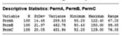
- a. Find the
range of the permeability measurements for Group A sandstone slices. Verify its value using the minimum and maximum values shown on the printout. - b. Find the standard deviation of the permeability measurements for Group A sandstone slices. Verify its value using the variance shown on the printout.
- c. Which condition (A, B, or C) has the more variable permeability data?
Want to see the full answer?
Check out a sample textbook solution
Chapter 2 Solutions
Statistics for Business and Economics (13th Edition)
Additional Math Textbook Solutions
Elementary Statistics Using Excel (6th Edition)
Elementary Statistics: Picturing the World (6th Edition)
Essential Statistics
Introduction to Statistical Quality Control
Elementary Statistics Using the TI-83/84 Plus Calculator, Books a la Carte Edition (4th Edition)
An Introduction to Mathematical Statistics and Its Applications (6th Edition)


- Repeat Example 5 when microphone A receives the sound 4 seconds before microphone B.arrow_forwardUrban Travel Times Population of cities and driving times are related, as shown in the accompanying table, which shows the 1960 population N, in thousands, for several cities, together with the average time T, in minutes, sent by residents driving to work. City Population N Driving time T Los Angeles 6489 16.8 Pittsburgh 1804 12.6 Washington 1808 14.3 Hutchinson 38 6.1 Nashville 347 10.8 Tallahassee 48 7.3 An analysis of these data, along with data from 17 other cities in the United States and Canada, led to a power model of average driving time as a function of population. a Construct a power model of driving time in minutes as a function of population measured in thousands b Is average driving time in Pittsburgh more or less than would be expected from its population? c If you wish to move to a smaller city to reduce your average driving time to work by 25, how much smaller should the city be?arrow_forwardFor the following table of data. x 1 2 3 4 5 6 7 8 9 10 y 0 0.5 1 2 2.5 3 3 4 4.5 5 a. draw a scatterplot. b. calculate the correlation coefficient. c. calculate the least squares line and graph it on the scatterplot. d. predict the y value when x is 11.arrow_forward
 Linear Algebra: A Modern IntroductionAlgebraISBN:9781285463247Author:David PoolePublisher:Cengage Learning
 Calculus For The Life SciencesCalculusISBN:9780321964038Author:GREENWELL, Raymond N., RITCHEY, Nathan P., Lial, Margaret L.Publisher:Pearson Addison Wesley,
 Functions and Change: A Modeling Approach to Coll...AlgebraISBN:9781337111348Author:Bruce Crauder, Benny Evans, Alan NoellPublisher:Cengage Learning
 Glencoe Algebra 1, Student Edition, 9780079039897...AlgebraISBN:9780079039897Author:CarterPublisher:McGraw Hill
 Algebra & Trigonometry with Analytic GeometryAlgebraISBN:9781133382119Author:SwokowskiPublisher:Cengage
 Trigonometry (MindTap Course List)TrigonometryISBN:9781337278461Author:Ron LarsonPublisher:Cengage Learning