
Videos
Total mobile data traffic.
The following graph shows the predicted monthly mobile data traffic for the years 2013–2018. Use these data in Exercises 25 and 26.
MOBILE DATA TRAFFIC
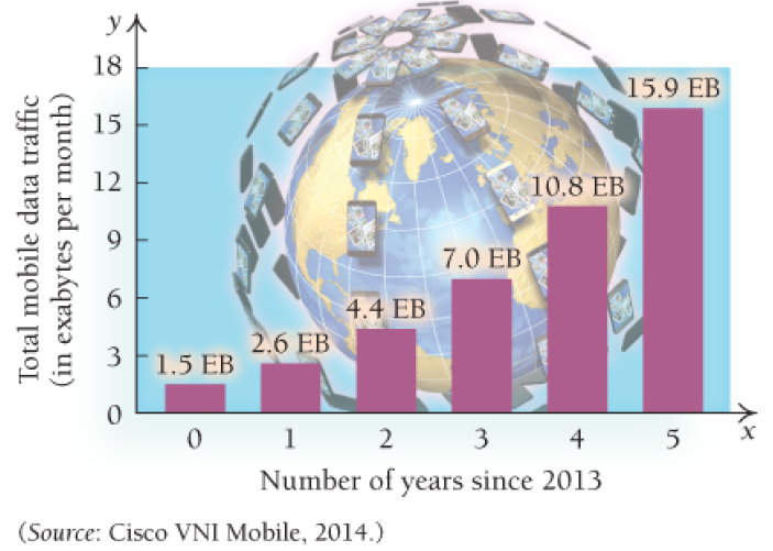
a. Use regression to fit an exponential function
Then convert the function to an exponential function, base e, using the fact that
b. What is the exponential growth rate, as a percentage?
c. Estimate the monthly mobile data traffic in 47.3% 2020.
d. When will the monthly mobile data traffic exceed 50 exabytes?
e. What is the doubling time for monthly mobile data traffic?
Want to see the full answer?
Check out a sample textbook solution
Chapter 3 Solutions
Calculus and Its Applications (11th Edition)
Additional Math Textbook Solutions
Calculus: Early Transcendentals (3rd Edition)
Calculus, Single Variable: Early Transcendentals (3rd Edition)
Precalculus: Concepts Through Functions, A Unit Circle Approach to Trigonometry (4th Edition)


- Exercises 93–94: Energy The following graph shows U.S. Energy consumption. 400 350 300 250 200 150 100 50 04 1970 1990 2010 Year 93. When was energy consumption increasing? 94. When was energy consumption decreasing? Energy (millions of Btu)arrow_forwardThe file P02_26.xlsx lists sales (in millions of dollars) of Dell Computer during the period 1987–1997 (where year 1 corresponds to 1987). Year Sales 1 69 2 159 3 258 4 389 5 546 6 890 7 2014 8 2873 9 3475 10 5296 11 7759 a. Fit a power and an exponential trend curve to these data. Which fits the data better? b. Use your part a answer to predict 1999 sales for Dell. c. Use your part a answer to describe how the sales of Dell have grown from year to year.arrow_forwardQ1. The table provided gives data on indexes of output per hour (X) and real compensation per hour (Y) for the business and nonfarm business sectors of the U.S. economy for 1960–2005. The base year of the indexes is 1992 = 100 and the indexes are seasonally adjusted. a. Plot Y against X for the two sectors separately. b. What is the economic theory behind the relationship between the two variables? Does the scattergram support the theory? c. Estimate the OLS regression of Y on X. Note: on the table ( 1. Output refers to real gross domestic product in the sector. 2. Wages and salaries of employees plus employers’ contributions for social insurance and private benefit plans. 3. Hourly compensation divided by the consumer price index for all urban consumers for recent quarters.) Thank you!arrow_forward
- National Debt The size of the total debt owed by the UnitedStates federal government continues to grow. In fact,according to the Department of the Treasury, the debt perperson living in the United States is approximately $53,000(or over $140,000 per U.S. household). The following datarepresent the U.S. debt for the years 2001–2014. Since thedebt D depends on the year y, and each input correspondsto exactly one output, the debt is a function of the year. SoD1y2 represents the debt for each year y. Source: www.treasurydirect.govDebt (billions Debt (billionsYear of dollars) Year of dollars)2001 5807 2008 10,0252002 6228 2009 11,9102003 6783 2010 13,5622004 7379 2011 14,7902005 7933 2012 16,0662006 8507 2013 16,7382007 9008 2014 17,824 (a) Plot the points 12001, 58072, 12002, 62282, and so on ina Cartesian plane.(b) Draw a line segment from the point 12001, 58072 to12006, 85072. What does the slope of this line segmentrepresent?(c) Find the average rate of change of the debt from 2002…arrow_forwardThe table shows the historical in-state tuition rates for the University of Kalamazoo. Use the data to answer the questions and round your answers to two decimal places. Academic year Rate of tuition for one semester 2008–2009 $3,812 2009–2010 $4,002 2010–2011 $4,441 2011–2012 $4,905 2012–2013 $5,181 What is the percentage increase in tuition from the 2008–2009 school year to the 2012–2013 school year?arrow_forwardproblen 1.4arrow_forward
- The table gives the yearly sales, S, of a retail store in years.arrow_forwardNielsen tracks the amount of time that people spend consuming media content across different platforms (digital, audio, television) in the United States. Nielsen has found that traditional television viewing habits vary based on the age of the consumer as an increasing number of people consume media through streaming devices.† The following data represent the weekly traditional TV viewing hours in 2016 for a sample of 14 people aged 18–34 and 12 people aged 35–49. (Round your answers to two decimal places.) Viewers aged 18–34 24.2 21.0 17.8 19.6 23.4 19.1 14.6 27.1 19.2 18.3 22.9 23.4 17.3 20.5 Viewers aged 35–49 24.9 34.9 35.8 31.9 35.4 29.9 30.9 36.7 36.2 33.8 29.5 30.8 (a) Compute the mean and median weekly hours of traditional TV viewed by those aged 18–34.arrow_forwardCell Phones Using the CTIA Wireless Survey for1985–2009, the number of U.S. cell phone subscribers (in millions) can be modeled byy = 0.632x2 - 2.651x + 1.209where x is the number of years after 1985.a. Graphically find when the number of U.S.subscribers was 301,617,000.b. When does the model estimate that the number ofU.S. subscribers would reach 359,515,000?c. What does the answer to (b) tell about this model?arrow_forward
- The average amount A (in pounds per person) of fish and shellfish consumed in the UnitedStates during the period 1992–2001 can be modeled by A = (3.2x + 260)/(52x + 3800) where x is the number of years since 1992.Rewrite the model so that it has only whole number coefficients. Then simplify the model.arrow_forwardSection 2.4: Chain Rule In Exercises 9–34, find the derivative of the function.arrow_forwardComplete Part D A recent issue of the AARP Bulletin reported that the average weekly pay for a woman with a high school degree is $520 (AARP Bulletin, January–February, 2010). Suppose you would like to determine if the average weekly pay for all working women is significantly greater than that for women with a high school degree. Data providing the weekly pay for a sample of 50 working women are available in the file named WeeklyPay. These data are consistent with the findings reported in the AARP article. Complete D null hyposthesis: H(o)=520Alternative hypothesis: H(a): greater then 520 sample mean=637.94 the test statistic = 5.62 p-value=0.00 Using a=.05, we would reject the null hypothesis. D. Repeat the hypothesis test using the critical value approach. 582 333 759 633 629 523 320 685 599 753 553 641 290 800 696 627 679 667 542 619 950 614 548 570 678 697 750 569…arrow_forward
 Calculus: Early TranscendentalsCalculusISBN:9781285741550Author:James StewartPublisher:Cengage Learning
 Thomas' Calculus (14th Edition)CalculusISBN:9780134438986Author:Joel R. Hass, Christopher E. Heil, Maurice D. WeirPublisher:PEARSON
 Calculus: Early Transcendentals (3rd Edition)CalculusISBN:9780134763644Author:William L. Briggs, Lyle Cochran, Bernard Gillett, Eric SchulzPublisher:PEARSON
 Calculus: Early TranscendentalsCalculusISBN:9781319050740Author:Jon Rogawski, Colin Adams, Robert FranzosaPublisher:W. H. Freeman
 Calculus: Early Transcendental FunctionsCalculusISBN:9781337552516Author:Ron Larson, Bruce H. EdwardsPublisher:Cengage Learning