
Videos
The depth of wetting of a soil is the depth to which water content will increase owing to external factors. The article “Discussion of Method for Evaluation of Depth of Wetting in Residential Areas” (J. Nelson, K. Chao, and D. Overton, Journal of Geotechnical and Geoenvironmental Engineering, 2011:293–296) discusses the relationship between depth of wetting beneath a structure and the age of the structure. The article presents measurements of depth of wetting, in meters, and the ages, in years, of 21 houses, as shown in the following table.
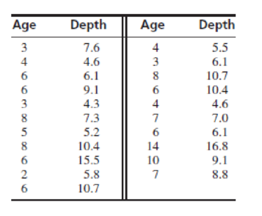
- a. Compute the least-squares line for predicting depth of wetting (y) from age (x).
- b. Identify a point with an unusually large x-value. Compute the least-squares line that results from deletion of this point.
- c. Identify another point which can be classified as an outlier. Compute the least-squares line that results from deletion of the outlier, replacing the point with the unusually large x-value.
- d. Which of these two points is more influential? Explain.
Want to see the full answer?
Check out a sample textbook solution
Chapter 7 Solutions
Statistics for Engineers and Scientists
Additional Math Textbook Solutions
Stats: Modeling the World Nasta Edition Grades 9-12
STATS:DATA+MODELS-W/DVD
Statistics Through Applications
Elementary Statistics Using The Ti-83/84 Plus Calculator, Books A La Carte Edition (5th Edition)
Introduction to Statistical Quality Control
Fundamentals of Statistics (5th Edition)


- Recently there has been increased use of stainless steel claddings in industrial settings. Claddings are used to finish the exterior walls of a building and help weatherproof the structure. To ensure the quality of claddings, it is essential to know how welding parameters impact the cladding process. The authors of “Mathematical Modeling of Weld Bead Geometry, Quality, and Productivity for Stainless Steel Claddings Deposited by FCAW” (J. Mater. Engr. Perform., 2012: 1862–1872) in vestigated how y 5 deposition rate was influenced by x1 = feed rate (Wf , in m/min) and x2 = welding speed (S, in cm/min). The following 22 observations correspond to the experiment condition where applied voltage was less than 30v: y: 2.718 3.881 2.773 3.924 2.740 3.870 x1 : 17.0 10.0 7.0 10.0 7.0 10.0 x 2 : 30 30 50 50 30 30 y: 2.847 3.901 2.204 4.454 3.324 3.319 x1 : 7.0 10.0 5.5 11.5 8.5 8.5 x2 : 50 50 40 40 40 20 The whole data and Question parts are attachedarrow_forwardThe article "Modeling Resilient Modulus and Temperature Correction for Saudi Roads" (H. Wahhab, I. Asi, and R. Ramadhan, Journal of Materials in Civil Engineering, 2001:298– 305) describes a study designed to predict the resilient modulus of pavement from physical properties. The following table presents data for the resilient modulus at 40°Cin10® kPa (y), the surface area of the aggregate in m²/kg (x1), and the softening point of the asphalt in °C (х). y X1 X2 1.48 5.77 60.5 1.70 7.45 74.2 2.03 8.14 67.6 2.86 8.73 70.0 2.43 7.12 64.6 3.06 6.89 65.3 2.44 8.64 66.2 1.29 6.58 64.1 3.53 9.10 68.6 1.04 8.06 58.8 1.88 5.93 63.2 1.90 8.17 62.1 1.76 9.84 68.9 2.82 7.17 72.2 1.00 7.78 54.1 The full quadratic model is y = + P,x, + PzX, + Pz*jXz + Pxx¡ + Bzx; + €. Which submodel of this full model do you believe is most appropriate? Justify your answer by fitting two or more models and comparing the results.arrow_forwardWrinkle recovery angle and tensile strength are the two most important characteristics for evaluating the performance of crosslinked cotton fabric. An increase in the degree of crosslinking, as determined by ester carboxyl band absorbance, improves the wrinkle resistance of the fabric (at the expense of reducing mechanical strength). The accompanying data on x = absorbance and y = wrinkle resistance angle was read from a graph in the paper "Predicting the Performance of Durable Press Finished Cotton Fabric with Infrared Spectroscopy".† x 0.115 0.126 0.183 0.246 0.282 0.344 0.355 0.452 0.491 0.554 0.651 y 334 342 355 363 365 372 381 392 400 412 420 Here is regression output from Minitab: Predictor Constant absorb S = 3.60498 Coef 321.878 156.711 SOURCE Regression Residual Error Total SE Coef 2.483 6.464 R-Sq = 98.5% DF 1 9 10 SS 7639.0 117.0 7756.0 T 129.64 24.24 0.000 0.000 R-Sq (adj) = 98.3% MS 7639.0 13.0 F P 587.81 (a) Does the simple linear regression model appear to be…arrow_forward
- Wrinkle recovery angle and tensile strength are the two most important characteristics for evaluating the performance of crosslinked cotton fabric. An increase in the degree of crosslinking, as determined by ester carboxyl band absorbance, improves the wrinkle resistance of the fabric (at the expense of reducing mechanical strength). The accompanying data on x = absorbance and y = wrinkle resistance angle was read from a graph in the paper "Predicting the Performance of Durable Press Finished Cotton Fabric with Infrared Spectroscopy".t 半 0.115 0.126 0.183 0.246 0.282 0.344 0.355 0.452 0.491 0.554 0.651 334 342 355 363 365 372 381 392 400 412 420 Here is regression output from Minitab: Predictor Coef SE Coef P Constant 321.878 2.483 129.64 0.000 absorb 156.711 6.464 24.24 0.000 S = 3.60498 R-Sq = 98.5% R-Są (adj) - 98.3% SOURCE DF MS F P Regression 1 7639.0 7639.0 587.81 0.000 Residual Error 9 117.0 13.0 Total 10 7756.0 (a) Does the simple linear regression model appear to be…arrow_forwardWrinkle recovery angle and tensile strength are the two most important characteristics for evaluating the performance of crosslinked cotton fabric. An increase in the degree of crosslinking, as determined by ester carboxyl band absorbance, improves the wrinkle resistance of the fabric (at the expense of reducing mechanical strength). The accompanying data on x = absorbance and y = wrinkle resistance angle was read from a graph in the paper "Predicting the Performance of Durable Press Finished Cotton Fabric with Infrared Spectroscopy".t x 0.115 0.126 0.183 0.246 0.282 0.344 0.355 0.452 0.491 0.554 0.651 y 334 342 355 363 365 372 381 400 392 412 420 Here is regression output from Minitab: Predictor Constant absorb S = 3.60498 Coef 321.878 156.711 SOURCE Regression Residual Error Total R-Sq= 98.5% DF SE Coef 2.483 6.464 1 9 10 SS 7639.0 117.0 7756..0 T 129.64 24.24 P 0.000 0.000. R-Sq (adj) 98.3% MS 7639.0 13.0 F 587.81 (a) Does the simple linear regression model appear to be appropriate?…arrow_forwardThis dataset includes measurements of soil temperature and soil respiration at three places along the riverbank (upper, mid, and lower; the upper site is far away from water and the lower site is close to water). Please help describe and interpret the results below:arrow_forward
- Foot ulcers are common problem for people with diabetes. Higher skin temperatures on the foot indicate an increased risk of ulcers. The article “An Intelligent Insole for Diabetic Patients with the Loss of Protective Sensation" (Kimberly Anderson, M.S. Thesis, Colorado School of Mines), reports measurements of temperatures, in °F, of both feet for 18 diabetic patients. The results are presented in the Table Q1. Table Ql: Measurements of temperatures, in °F of left foot Vs right foot for 18 diabetic patients Left Foot Right Foot Left Foot Right Foot 80 80 76 81 85 85 89 86 80 86 75 87 82 88 78 78 89 87 80 81 87 82 87 82 78 78 86 85 88 89 76 80 89 90 88 89 (d) Test the slope, ß1 = 1 at 5% level of significance. (e) Calculate the coefficient of correlation r and r2 and then interpret their valuesarrow_forwardPlease use the accompanying Excel data set or accompanying Text file data set when completing the following exercise. An article in Wood Science and Technology, "Creep in Chipboard, Part 3: Initial Assessment of the Influence of Moisture Content and Level of Stressing on Rate of Creep and Time to Failure" (1981, Vol. 15, pp. 125-144) studied the deflection (mm) of particleboard from stress levels of relative humidity. Assume that the two variables are related according to the simple linear regression model. The data are shown below x = Stress level (%) 54 54 61 61 68 68 75 75 75 y = Deflection (mm) 16.473 18.693 14.305 15.121 13.505 11.64 11.168 12.534 11.224 a. Calculate the least square estimates of the intercept (a) and slope (b). What is the estimate of o (c)? b. Find the estimate of the mean deflection if the stress level can be limited to 61% (d). c. Estimate the change in the mean deflection associated with a 7% increment in stress level (e). (a) i (Round your answer to 2…arrow_forwardPlease use the accompanying Excel data set or accompanying Text file data set when completing the following exercise. An article in Wood Science and Technology, "Creep in Chipboard, Part 3: Initial Assessment of the Influence of Moisture Content and Level of Stressing on Rate of Creep and Time to Failure" (1981, Vol. 15, pp. 125-144) studied the deflection (mm) of particleboard from stress levels of relative humidity. Assume that the two variables are related according to the simple linear regression model. The data are shown below x = Stress level (%) 54 54 61 61 68 68 75 75 75 y = Deflection (mm) 16.473 18.693 14.305 15.121 13.505 11.64 11.168 12.534 11.224 a. Calculate the least square estimates of the intercept (a) and slope (b). What is the estimate of o² (c)? b. Find the estimate of the mean deflection if the stress level can be limited to 66% (d). c. Estimate the change in the mean deflection associated with a 8% increment in stress level (e). (a) i (Round your answer to 2…arrow_forward
- The article "Characteristics and Trends of River Discharge into Hudson, James, and Ungava Bays, 1964-2000" (S. Dery, M. Stieglitz, et al., Journal of Climate, 2005:2540-2557) presents measurements of discharge rate x (in kmlyr) andpeakflow y (in m/s) for 42 rivers that drain into the Hudson, James, and Ungava Bays. The data are shown in the following table: Discharge Peak Flow 94.24 4110.3 66.57 4961.7 59.79 10275.5 48.52 6616.9 40.00 7459.5 32.30 2784.4 31.20 3266.7 30.69 4368.7 26.65 1328.5 22.75 4437.6 21.20 1983.0 20.57 1320.1 19.77 1735.7 18.62 1944.1 17.96 3420.2 17.84 2655.3 16.06 3470.3 1561.6 14.69 11.63 869.8 11.19 936.8 11.08 1315.7 10.92 1727.1 9.94 768.1 7.86 483.3arrow_forwardThe article "Effect of Granular Subbase Thickness on Airfield Pavement Structural Response" (K. Gopalakrishnan and M. Thompson, Journal of Materials in Civil Engineering, 2008:331-342) presents a study of the amount of surface deflection caused by aircraft landing on an airport runway. A load of 160 kN was applied to a runway surface, and the amount of deflection in mm (y) was measured at various distances in m (x) from the point of application. The results are presented in the following table. y 0.000 3.24 0.305 2.36 0.610 1.42 0.914 0.87 1.219 0.54 1.524 0.34 1.830 0.24 a. Fit the linear model y = Bo + B1x + ɛ. For each coefficient, test the hypothesis that the coefficient is equal to 0. b. Fit the quadratic model y = Bo + Bịx + B2x² + ɛ. For each coefficient, test the hypothesis that the coefficient is equal to 0. %3D Fit the cubic model y = Bo + B1x + B2x? + B3x + E. For each coefficient, test the C. hypothesis that the coefficient is equal to 0. d. Which of the models in parts (a)…arrow_forwardSpecial dyes have been developed that only bind to DNA. The intensity of the color is directly related to the quantity of DNA present in the cell. A haploid cell would have a “low” amount of color, a cell in G1 would have a “medium” amount of color, and a cell in M phase would have a “high” amount of color. Is this sort of assessment quantitative, qualitative or semi-quantitative? Justify your reasoning.arrow_forward
 Linear Algebra: A Modern IntroductionAlgebraISBN:9781285463247Author:David PoolePublisher:Cengage Learning