Statistics for Business and Economics (13th Edition)
13th Edition
ISBN: 9780134506593
Author: James T. McClave, P. George Benson, Terry Sincich
Publisher: PEARSON
expand_more
expand_more
format_list_bulleted
Concept explainers
Videos
Textbook Question
Chapter 11, Problem 11.115ACI
Evaluating a truck weigh-in-motion program. The Minnesota Department of Transportation installed a state-of-the-art weigh-in-motion scale in the concrete surface of the eastbound lanes of Interstate 494 in Bloomington, Minnesota. After installation. a study was undertaken to determine whether the scale’s readings correspond to the static weights of the vehicles being monitored. (Studies of this type are known as calibration studies.) After some preliminary comparisons using a two-axle, six-tire truck carrying different loads (see the accompanying table), calibration adjustments were made in the software of the weigh-in-motion system, and the scales were reevaluated.
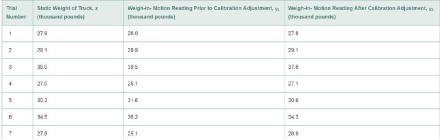
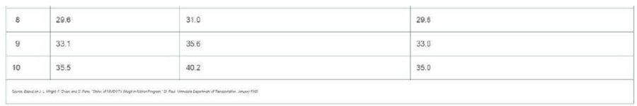
- a. Construct two
scatterplots . one of y1 versus x and the other of y2 versus x. - b. Use the scatterplots of part a to evaluate the performance of the weigh-in-motion scale both before and after the calibration adjustment.
- c. Calculate the
correlation coefficient for both sets of data and Interpret their values. Explain how these correlation coefficients can be used to evaluate the weigh-in-motion scale. - d. Suppose the sample correlation coefficient for y1 and x was 1. Could this happen if the static weights and the weigh-in-motion readings disagreed? Explain.
Expert Solution & Answer
Want to see the full answer?
Check out a sample textbook solution
Students have asked these similar questions
A study was conducted at a local college to analyze the average cumulative GPA’s of students who graduated last year. Fill in the letter of the phrase that best describes each of the items below. The average cumulative GPA of students in the study who graduated from the college last year is?
a.
Data
b.
Sample
c.
Population
d.
Statistic
e.
Variable
f.
Parameter
A semiconductor manufacturer produces devices used as central processing units in personal computers.
The speed of two model devices, measured in megahertz, is important because it determines the price that
the manufacturer can charge for the devices. The following data presents the measurement on 20 devices
each for the two models.
Model A:
680
670
710
669
669
719
699
722
663
658
634
720
690
677
700
718
690
681
702
Model B:
652
720
660
695
701
724
668
698
668
660
680
739
717
727
653
637
660
693
679
a. Which of the two models is relatively faster? What is your basis for stating such?
b. If you were to choose which between the two models you are going to use as central processing unit in
a personal computer, which would it be and why? Support your answer statistically.
A professor at the University of Iowa was interested in evaluating whether domestic dispute calls were more dangerous to officers than other types of calls. Collecting information on call for service and whether the call resulted in officer injury. The data is displayed in the contingency table below.
Type of Call
Domestic Dispute
Not a Domestic Dispute
Officer Injury
No
128
675
Yes
245
786
Using the information to complete Table 1 and answer the questions below.
Table 1. Chi-square (4 points, 1 per column)
Category
Observed
Expected
O – E
(O – E)2
(O – E)2/E
No, Domestic
128
No, Not Domestic
675
Yes, Domestic
245
Yes, Not Domestic
786
What is the scale of measurement of the dependent variable?
What is the value for the chi-square?
Using an alpha level of 0.05, what is the critical…
Chapter 11 Solutions
Statistics for Business and Economics (13th Edition)
Ch. 11.1 - In each case, graph the line that passes through...Ch. 11.1 - Give the slope and y-intercept for each of the...Ch. 11.1 - The equation for a straight line (deterministic...Ch. 11.1 - Refer to Exercise 11.3. Find the equations of the...Ch. 11.1 - Plot the following lines: a. y 4 + x b. y = 5 2x...Ch. 11.1 - Give the slope and y-intercept for each of the...Ch. 11.1 - Prob. 11.7LMCh. 11.1 - Prob. 11.8LMCh. 11.1 - If a straight-line probabilistic relationship...Ch. 11.1 - Congress voting on women's issues. The American...
Ch. 11.1 - Best-paid CEOs. Refer to Glassdoor Economic...Ch. 11.1 - Estimating repair and replacement costs of water...Ch. 11.1 - Forecasting movie revenues with Twitter. A study...Ch. 11.2 - The following table is similar to Table 11.2.It is...Ch. 11.2 - Refer to Exercise 11.14. After the least squares...Ch. 11.2 - Construct a scatterplot for the data in the...Ch. 11.2 - Consider the following pairs of measurements: a....Ch. 11.2 - Use the applet Regression by Eye to explore the...Ch. 11.2 - In business, do nice guys finish first or last?...Ch. 11.2 - State Math SAT scores. Refer to the data on...Ch. 11.2 - Lobster fishing study. Refer to the Bulletin of...Ch. 11.2 - Repair and replacement costs of water pipes. Refer...Ch. 11.2 - Joint Strike Fighter program. The Joint Strike...Ch. 11.2 - Software millionaires and birthdays. In Outliers:...Ch. 11.2 - Prob. 11.24ACICh. 11.2 - Ranking driving performance of professional...Ch. 11.2 - Sweetness of orange juice. The quality of the...Ch. 11.2 - Forecasting movie revenues with Twitter. Marketers...Ch. 11.2 - Charisma of top-level leaders. According to a...Ch. 11.2 - Ran kings of research universities. Refer to the...Ch. 11.2 - Prob. 11.30ACACh. 11.3 - Visually compare the scatterplots shown below. If...Ch. 11.3 - Calculate SSE and s2 for each of the following...Ch. 11.3 - Suppose you fit a least squares line to 26 data...Ch. 11.3 - Refer to Exercise 11.14 (p. 629). Calculate SSE,...Ch. 11.3 - Do nice guys really finish last in business? Refer...Ch. 11.3 - State Math SAT scores. Refer to the simple linear...Ch. 11.3 - Prob. 11.37ACBCh. 11.3 - Prob. 11.38ACBCh. 11.3 - Prob. 11.39ACBCh. 11.3 - Prob. 11.40ACICh. 11.3 - Prob. 11.41ACICh. 11.3 - Sweetness of orange juice. Refer to the study of...Ch. 11.3 - Rankings of research universities. Refer to the...Ch. 11.3 - Life tests of cutting tools. To Improve the...Ch. 11.4 - Construct both a 95% and a 90% confidence interval...Ch. 11.4 - Consider the following pairs of observations: a....Ch. 11.4 - Refer to Exercise 11.46. Construct an 80% and a...Ch. 11.4 - Do the accompanying data provide sufficient...Ch. 11.4 - State Math SAT Scores. Refer to the SPSS simple...Ch. 11.4 - Lobster fishing study. Refer to the Bulletin of...Ch. 11.4 - Prob. 11.51ACBCh. 11.4 - Prob. 11.52ACBCh. 11.4 - Estimating repair and replacement costs of water...Ch. 11.4 - Prob. 11.54ACBCh. 11.4 - Prob. 11.55ACICh. 11.4 - Beauty and electoral success. Are good looks an...Ch. 11.4 - Prob. 11.57ACICh. 11.4 - Prob. 11.58ACICh. 11.4 - Prob. 11.59ACICh. 11.4 - Prob. 11.60ACICh. 11.4 - Rankings of research universities. Refer to the...Ch. 11.4 - Prob. 11.62ACACh. 11.4 - Does elevation impact hitting performance in...Ch. 11.5 - Explain what each of the following sample...Ch. 11.5 - Describe the slope of the least squares line if a....Ch. 11.5 - Construct a scatterplot for each data set. Then...Ch. 11.5 - Calculate r2 for the least squares line in each of...Ch. 11.5 - Use the applet Correlation by Eye to explore the...Ch. 11.5 - In business, do nice guys finish first or last?...Ch. 11.5 - Going for it on fourth-down in the NFL Each week...Ch. 11.5 - Lobster fishing study. Refer to the Bulletin of...Ch. 11.5 - RateMyProfessors.com. A popular Web site among...Ch. 11.5 - Last name and acquisition timing. Refer to the...Ch. 11.5 - Women in top management. An empirical analysis of...Ch. 11.5 - Prob. 11.74ACICh. 11.5 - Prob. 11.75ACICh. 11.5 - Prob. 11.76ACICh. 11.5 - Prob. 11.77ACICh. 11.5 - Prob. 11.78ACICh. 11.5 - Evaluation of an imputation method for missing...Ch. 11.5 - Prob. 11.80ACICh. 11.5 - Prob. 11.81ACACh. 11.6 - Consider the followings of measurements: a...Ch. 11.6 - Consider the pairs of measurements shown in the...Ch. 11.6 - In fitting a least squares line to n = 10 data...Ch. 11.6 - Prob. 11.86ACBCh. 11.6 - Prob. 11.87ACBCh. 11.6 - Prob. 11.88ACBCh. 11.6 - Prob. 11.89ACBCh. 11.6 - Prob. 11.90ACBCh. 11.6 - Prob. 11.91ACICh. 11.6 - Ranking driving performance of professional...Ch. 11.6 - Spreading rate of spilled liquid Refer to the...Ch. 11.6 - Removing nitrogen from toxic wastewater. Highly...Ch. 11.6 - Predicting quit rates In manufacturing The reasons...Ch. 11.6 - Life tests of cutting tools Refer to the data...Ch. 11.7 - Prices of recycled materials. Prices of recycled...Ch. 11.7 - Thickness of dust on solar cells. The performance...Ch. 11.7 - Management research In Africa. The editors of the...Ch. 11.7 - An MBAs work-life balance. The importance of...Ch. 11 - In fitting a least squares line ton= 15 data...Ch. 11 - Consider the following sample data. a. Construct a...Ch. 11 - Consider the following 10 data points. a. Plot the...Ch. 11 - Drug controlled-release rate study. The effect of...Ch. 11 - Metaskills and career management. Effective...Ch. 11 - Burnout of human services professionals. Emotional...Ch. 11 - Retaliation against company whistle-blowers....Ch. 11 - Extending the life of an aluminum smelter pot. An...Ch. 11 - Diamonds sold at retail. Refer to the Journal of...Ch. 11 - Sports news on local TV broadcasts. The Sports...Ch. 11 - Evaluating managerial success. An observational...Ch. 11 - Doctors and ethics. Refer to the Journal of...Ch. 11 - FCAT scores and poverty. In the state of Florida,...Ch. 11 - Monetary values of NFL teams. Refer to the Forbes...Ch. 11 - Evaluating a truck weigh-in-motion program. The...Ch. 11 - Energy efficiency of buildings. Firms conscious of...Ch. 11 - Forecasting managerial needs. Managers are an...Ch. 11 - Prob. 11.118ACACh. 11 - Prob. 11.119CTCCh. 11 - Prob. 11.120CTC
Knowledge Booster


Learn more about
Need a deep-dive on the concept behind this application? Look no further. Learn more about this topic, statistics and related others by exploring similar questions and additional content below.Similar questions
- A paper investigated the driving behavior of teenagers by observing their vehicles as they left a high school parking lot and then again at a site approximately mile from the school. Assume that it is reasonable to regard the teen drivers in this study as representative of the population of teen drivers. Amount by Which Speed Limit Was Exceeded Male Female Driver Driver 1.4 -0.1 1.2 0.4 0.9 1.1 2.1 0.7 0.7 1.1 1.3 1.2 0.1 1.3 0.9 0.6 0.5 2.1 0.5 (a) Use a .01 level of significance for any hypothesis tests. Data consistent with summary quantities appearing in the paper are given in the table. The measurements represent the difference between the observed vehicle speed and the posted speed limit (in miles per hour) for a sample of male teenage drivers and a sample of female teenage drivers. (Use umales - Hiemales: Round your test statistic to two decimal places. Round your degrees of freedom down to the nearest whole number. Round your p-value to three decimal places.) t = 2.969 df = 18…arrow_forwardA paper investigated the driving behavior of teenagers by observing their vehicles as they left a high school parking lot and then again at a site approximately mile from the school. Assume that it is reasonable to regard the teen drivers in this study as representative of the population of teen drivers. Amount by Which Speed Limit Was Exceeded Male Female Driver Driver 1.4 -0.3 1.2 0.6 0.9 1.1 2.1 0.7 0.7 1.1 1.3 1.2 3 0.1 1.3 0.9 0.6 0.5 2.1 0.5 (a) Use a .01 level of significance for any hypothesis tests. Data consistent with summary quantities appearing in the paper are given in the table. The measurements represent the difference between the observed vehicle speed and the posted speed limit (in miles per hour) for a sample of male teenage drivers and a sample of female teenage drivers. (Use umales - Hfemales: Round your test statistic to two decimal places. Round your degrees of freedom down to the nearest whole number. Round your p-value to three decimal places.) t = df = P = (b)…arrow_forwardA salesperson purchased an automobile that was advertised as averaging 27 miles/gallon in the city and 38 miles/gallon on the highway. A recent sales trip that covered 1300 miles required 40 gallons of gasoline. Assuming that the advertised mileage estimates were correct, how many highway miles were driven on the trip? hint: even though you're asked to find highway miles , I recommend having your variables represent the number of gallons of gasoline used in the city and on the highway Number of highway milesarrow_forward
- The height of 10 skeletons (denoted by the variable stature) and the length of the middle metacarpal bone were measured (the metacarpal bones are in the hand between the wrist and fingers). The skeletal height is measured in centimeters and the metacarpal length in millimeters. The scatterplot is given below. X 1. Describe what the scatterplot tells you about the direction, form, and strength of the relationship. stature (cm) 180.0 172.5 165.0 157.5 - . + + 51 39 45 metacarpal size (mm) 2. In this setting, is there a definite explanatory variable and response variable? Justify your answer. 3. Estimate the correlation between metacarpal length and stature. No calculations are necessary. 4. If the height and metacarpal length of the skeletons had been measured in inches, instead of centimeters and millimeters, how would the correlation between stature and metacarpal length for these 10 skeletons have been affected? Explain. 5. One of these skeletons (identified by the X) had a metacarpal…arrow_forwardYou may need to use the appropriate technology to answer this question. An automobile dealer conducted a test to determine if the time in minutes needed to complete a minor engine tune-up depends on whether a computerized engine analyzer or an electronic analyzer is used. Because tune-up time varies among compact, intermediate, and full-sized cars, the three types of cars were used as blocks in the experiment. The data obtained follow. Analyzer computerized electronic Car compact 50 41 Intermediate 56 45 Full Sized 62 46 Use ? = 0.05 to test for any significant differences. State the null and alternative hypotheses. H0: ?Computerized = ?ElectronicHa: ?Computerized ≠ ?ElectronicH0: ?Computerized ≠ ?ElectronicHa: ?Computerized = ?Electronic H0: ?Computerized = ?Electronic = ?Compact = ?Intermediate = ?Full-sizedHa: Not all the population means are equal.H0: ?Compact = ?Intermediate = ?Full-sizedHa: ?Compact ≠ ?Intermediate ≠ ?Full-sizedH0:…arrow_forwardyour car is more crowded than you think. table 5.8 reports results from a 1969 personal transportation survey on "home-to-work" trips in metropolitan areas. The survey stated that the average car occupancy was 1.4 people. check that calculation.arrow_forward
- You may need to use the appropriate technology to answer this question. An automobile dealer conducted a test to determine if the time in minutes needed to complete a minor engine tune-up depends on whether a computerized engine analyzer or an electronic analyzer is used. Because tune-up time varies among compact, intermediate, and full-sized cars, the three types of cars were used as blocks in the experiment. The data obtained follow. Analyzer Computerized Electronic Compact 50 41 Car Intermediate 54 44 Full-sized 64 47 Use a = 0.05 to test for any significant differences. State the null and alternative hypotheses. O Ho: MCompact = "Intermediate = HFull-sized H: "Compact * "Intermediate * "Full-sized O Ho: "Compact * "Intermediate * HFull-sized H: "Compact "Intermediate = "Full-sized O Ho: Computerized = HElectronic H: "Computerized * HElectronic O Ho: "Computerized = HElectronic = "Compact = Intermediate = Full-sized H: Not all the population means are equal. O Ho: HComputerized *…arrow_forward1. calculate skewness from the dataarrow_forwardThe NTSB wants to estimate the difference between the average stopping distance for a car traveling 40 MPH on wet versus dry pavement. Ten vehicles were used for the study where each vehicle was driven at 40 MPH and came to a sudden stop on both wet pavement and dry pavement. The stopping distance was measured (feet) for each pavement condition and the data is shown below followed by Minitab output with the CI. Vehicle 1 2 3 4 5 6 7 8 9 10 Wet 107 101 109 112 105 106 111 108 98 116 Dry 72 69 74 73 72 72 74 74 67 79 Estimation for Paired Difference Mean StDev SE Mean 95% CI forμ_difference 34.700 2.452 0.775 (32.946, 36.454) a. Interpret the 95% CI.b. What assumption is needed for this CI to be valid?arrow_forward
- Because of safety considerations, in May 2003 the Federal Aviation Administration (FAA) changed its guidelines for how small commuter airlines must estimate passenger weights. Under the old rule, airlines used 180 pounds as a typical passenger weight (including carry-on luggage) in warm months and 185 pounds as a typical weight in cold months. A journal reported that an airline conducted a study to estimate average passenger plus carry-on weights. They found an average summer weight of 183 pounds and a winter average of 190 pounds. Suppose that each of these estimates was based on a random sample of 100 passengers and that the sample standard deviations were 18 pounds for the summer weights and 21 pounds for the winter weights. n USE SALT (a) Construct a 95% confidence interval for the mean summer weight (including carry-on luggage) of this airline's passengers. (Use technology to calculate the critical value. Round your answers to three decimal places.) Interpret a 95% confidence…arrow_forwardBecause of safety considerations, in May 2003 the Federal Aviation Administration (FAA) changed its guidelines for how small commuter airlines must estimate passenger weights. Under the old rule, airlines used 180 pounds as a typical passenger weight (including carry-on luggage) in warm months and 185 pounds as a typical weight in cold months. A journal reported that an airline conducted a study to estimate average passenger plus carry-on weights. They found an average summer weight of 183 pounds and a winter average of 190 pounds. Suppose that each of these estimates was based on a random sample of 100 passengers and that the sample standard deviations were 15 pounds for the summer weights and 21 pounds for the winter weights. (a) Construct a 95% confidence interval for the mean summer weight (including carry-on luggage) of this airline's passengers. (Use technology to calculate the critical value. Round your answers to three decimal places.) ( , )…arrow_forwardThe owner of a moving company typically has their most experienced manager predict the total number of labor hours that will be required to complete an upcoming move. The approach has proven useful in the past, but the owner has their business objective of developing a more accurate method of predicting labor hours. In a preliminary effort to provide a more accurate method, the owner has decided to use the number of cubic feet moved as the independent variable and has collected data for 36 moves. The data is seen below: Hours Feet 24.00 545 13.50 400 26.25 562 25.00 540 9.00 220 20.00 344 22.00 569 11.25 340 50.00 900 12.00 285 38.75 865 40.00 831 19.50 344 18.00 360 28.00 750 27.00 650 21.00 415 15.00 275 25.00 557 45.00 1028 29.00 793 21.00 523 22.00 564 16.50 312 37.00 757 32.00 600 34.00 796 25.00 577…arrow_forward
arrow_back_ios
SEE MORE QUESTIONS
arrow_forward_ios
Recommended textbooks for you
 Glencoe Algebra 1, Student Edition, 9780079039897...AlgebraISBN:9780079039897Author:CarterPublisher:McGraw Hill
Glencoe Algebra 1, Student Edition, 9780079039897...
Algebra
ISBN:9780079039897
Author:Carter
Publisher:McGraw Hill
Statistics 4.1 Point Estimators; Author: Dr. Jack L. Jackson II;https://www.youtube.com/watch?v=2MrI0J8XCEE;License: Standard YouTube License, CC-BY
Statistics 101: Point Estimators; Author: Brandon Foltz;https://www.youtube.com/watch?v=4v41z3HwLaM;License: Standard YouTube License, CC-BY
Central limit theorem; Author: 365 Data Science;https://www.youtube.com/watch?v=b5xQmk9veZ4;License: Standard YouTube License, CC-BY
Point Estimate Definition & Example; Author: Prof. Essa;https://www.youtube.com/watch?v=OTVwtvQmSn0;License: Standard Youtube License
Point Estimation; Author: Vamsidhar Ambatipudi;https://www.youtube.com/watch?v=flqhlM2bZWc;License: Standard Youtube License