Elementary Statistics ( 3rd International Edition ) Isbn:9781260092561
3rd Edition
ISBN: 9781259969454
Author: William Navidi Prof.; Barry Monk Professor
Publisher: McGraw-Hill Education
expand_more
expand_more
format_list_bulleted
Concept explainers
Videos
Textbook Question
Chapter 2.3, Problem 32E
More gold: The following time series plot presents the number of countries participating in the Summer Olympic games in each Olympic year from 1952 through 2016.
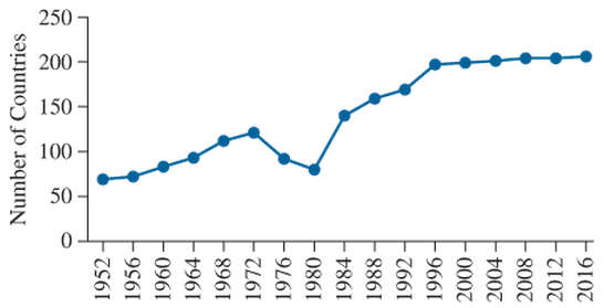
Refer to Exercise 30. Someone says “Although the number of gold medals won by the United States didn’t change much from 1952 to 1972, the performance of the United States steadily improved during that period.” Which feature of the plot of the number of participating countries justifies that statement?
Expert Solution & Answer
Want to see the full answer?
Check out a sample textbook solution
Students have asked these similar questions
The data shown indicate the number of wins and the number of points scored for teams in a hockey league. Use a TI-83 Plus/TI-84 Plus calculator to construct
the scatter plot.
No. of wins, x
11
6
5
9
10
9
7
8
No. of points, y
15
26
29
20
16
18
24
23
Send data to Excel
Part: 0 / 2
Part 1 of 2
Select the correct graph.
Graph A
Graph B
y
y
30+
30
25 -
25
20-
20
15-
15
10-
10-
In 2000, the population of a town was 46,020. By 2002 the population had increased to 52,070. Assuming the towns population is increasing
linearly answer the following questions
a. What is the population of the town by 2006?
b. What year will the towns population reach 75,000?
a.
type your answer..
b. type your answer.
The tables show the cat population on two islands over several years. Describe
mathematically, as precisely as you can, how the cat population on each island is
changing.
year
1.
2
number of cats on Meow Island 2
6.
18
54
162
year
1
4
number of cats on Purr Island
2
6
10
14
18
6
Chapter 2 Solutions
Elementary Statistics ( 3rd International Edition ) Isbn:9781260092561
Ch. 2.1 - In Exercises 5-8, fill in each blank with the...Ch. 2.1 - In Exercises 5-8, fill in each blank with the...Ch. 2.1 - In Exercises 5-8, fill in each blank with the...Ch. 2.1 - In Exercises 5-8, fill in each blank with the...Ch. 2.1 - In Exercises 9—12, determine whether the...Ch. 2.1 - In Exercises 9—12, determine whether the...Ch. 2.1 - In Exercises 9—12, determine whether the...Ch. 2.1 - In Exercises 9—12, determine whether the...Ch. 2.1 - The following bar graph presents the average...Ch. 2.1 - The most common blood typing system divides human...
Ch. 2.1 - Following is a pie chart that presents the...Ch. 2.1 - Government spending: The following pie chart...Ch. 2.1 - U.S. population: The following side-by-side bar...Ch. 2.1 - Super Bowl: The following side-by-side bar graph...Ch. 2.1 - Smartphone sales: The following frequency...Ch. 2.1 - Popular video games: The following frequency...Ch. 2.1 - More smartphones: Using the data in Exercise 19:...Ch. 2.1 - More video games: Using the data in Exercise 20:...Ch. 2.1 - Hospital admissions: The following frequency...Ch. 2.1 - World population: Following are the populations of...Ch. 2.1 - Ages of video garners: The Nielsen Company...Ch. 2.1 - How secure is your job? In a survey, employed...Ch. 2.1 - Back up your data: In a survey commissioned by the...Ch. 2.1 - Education levels: The following frequency...Ch. 2.1 - Twitter followers: The following frequency...Ch. 2.1 - Music sales: The following frequency distribution...Ch. 2.1 - Keeping up with the Kardashians: The following...Ch. 2.1 - Bought a new car lately? The following table...Ch. 2.1 - Bought a new- truck lately? The following table...Ch. 2.1 - Happy Halloween: The following table presents...Ch. 2.1 - Native languages: The following frequency...Ch. 2.1 - Proportion of females: Following are the...Ch. 2.2 - Prob. 5ECh. 2.2 - In Exercises 5—8, fill in each blank with the...Ch. 2.2 - In Exercises 5—8, fill in each blank with the...Ch. 2.2 - In Exercises 5—8, fill in each blank with the...Ch. 2.2 - In Exercises 9—12, determine whether the...Ch. 2.2 - In Exercises 9—12, determine whether the...Ch. 2.2 - In Exercises 9—12, determine whether the...Ch. 2.2 - In Exercises 9—12, determine whether the...Ch. 2.2 - In Exercises 13—16, classify the histogram as...Ch. 2.2 - In Exercises 13—16, classify the histogram as...Ch. 2.2 - In Exercises 13—16, classify the histogram as...Ch. 2.2 - In Exercises 13—16, classify the histogram as...Ch. 2.2 - In Exercises 17 and 18, classify the histogram as...Ch. 2.2 - In Exercises 17 and 18, classify the histogram as...Ch. 2.2 - Student heights: The following frequency histogram...Ch. 2.2 - Trained rats: Forty rats were trained to run a...Ch. 2.2 - Cholesterol: The following histogram shows the...Ch. 2.2 - Blood pressure: The following histogram shows the...Ch. 2.2 - Olympic athletes: The following frequency...Ch. 2.2 - Hows the weather? The following relative frequency...Ch. 2.2 - Skewed which way? For which of the following data...Ch. 2.2 - Skewed which way? For which of the following data...Ch. 2.2 - Batting average: The following frequency...Ch. 2.2 - Batting average: The following frequency...Ch. 2.2 - Time spent playing video games: A sample of 200...Ch. 2.2 - Murder, she wrote: The following frequency...Ch. 2.2 - BMW prices: The following table presents the...Ch. 2.2 - Geysers: The geyser Old Faithful in Yellowstone...Ch. 2.2 - Hail to the chief: There have been 58 presidential...Ch. 2.2 - Internet radio: The following table presents the...Ch. 2.2 - Brothers and sisters: Thirty students in a...Ch. 2.2 - Cough, cough: The following table presents the...Ch. 2.2 - Prob. 37ECh. 2.2 - Prob. 38ECh. 2.2 - Prob. 39ECh. 2.2 - Prob. 40ECh. 2.2 - Frequency polygon: Using the data in Exercise 29:...Ch. 2.2 - Prob. 42ECh. 2.2 - Ogive: Using the data in Exercise 27: Compute the...Ch. 2.2 - Ogive: Using the data in Exercise 28: Compute the...Ch. 2.2 - Ogive: Using the data in Exercise 29: Compute the...Ch. 2.2 - Prob. 46ECh. 2.2 - Prob. 47ECh. 2.2 - Prob. 48ECh. 2.2 - Prob. 49ECh. 2.2 - Prob. 50ECh. 2.2 - Prob. 51ECh. 2.2 - Prob. 52ECh. 2.2 - Frequencies and relative frequencies: The...Ch. 2.3 - In Exercises 3—6, fill in each blank with the...Ch. 2.3 - In Exercises 3—6, fill in each blank with the...Ch. 2.3 - In Exercises 3—6, fill in each blank with the...Ch. 2.3 - In Exercises 3—6, fill in each blank with the...Ch. 2.3 - Prob. 7ECh. 2.3 - In Exercises 7—10, determine whether the...Ch. 2.3 - In Exercises 7—10, determine whether the...Ch. 2.3 - In Exercises 7—10, determine whether the...Ch. 2.3 - Construct a stem-and-leaf plot for the following...Ch. 2.3 - Construct a stem-and-leaf plot for the following...Ch. 2.3 - List the data in the following stem-and-leaf plot....Ch. 2.3 - List the data in the following stein-and-leaf...Ch. 2.3 - Construct a dotplot for the data in Exercise 11.Ch. 2.3 - Prob. 16ECh. 2.3 - BMW prices: The following table presents the...Ch. 2.3 - Hows the weather? The following table presents the...Ch. 2.3 - Air pollution: The following table presents...Ch. 2.3 - Technology salaries: The following table presents...Ch. 2.3 - Tennis and golf: Following are the ages of the...Ch. 2.3 - Pass the popcorn: Following are the running times...Ch. 2.3 - More weather: Construct a dotplot for the data in...Ch. 2.3 - Prob. 24ECh. 2.3 - Looking for a job: The following table presents...Ch. 2.3 - Prob. 26ECh. 2.3 - Military spending: The following table presents...Ch. 2.3 - Prob. 28ECh. 2.3 - Dining out: The following time-series plot...Ch. 2.3 - Prob. 30ECh. 2.3 - Prob. 31ECh. 2.3 - More gold: The following time series plot presents...Ch. 2.3 - Prob. 33ECh. 2.3 - Prob. 34ECh. 2.3 - Vote: The following time-series plot presents the...Ch. 2.3 - Arctic ice sheet: The following table presents the...Ch. 2.3 - Prob. 37ECh. 2.4 - In Exercises 3 and 4, fill in each blank with the...Ch. 2.4 - In Exercises 3 and 4, fill in each blank with the...Ch. 2.4 - CD sales decline: Sales of CDs have been declining...Ch. 2.4 - Music sales: The following time-series plot and...Ch. 2.4 - Stock market prices: The Dow Jones Industrial...Ch. 2.4 - Save your money: In 2007, U.S. residents saved...Ch. 2.4 - Ill take mine with mustard: The following bar...Ch. 2.4 - Stream or download? The following bar graph...Ch. 2.4 - Female senators: Of the 100 members of the United...Ch. 2.4 - Age at marriage: Data compiled by the U.S. Census...Ch. 2.4 - College degrees: Both of the following time-series...Ch. 2.4 - Food expenditures: Both of the following...Ch. 2.4 - Prob. 15ECh. 2 - Following is the list of letter grades for...Ch. 2 - Prob. 2CQCh. 2 - Construct a frequency bar graph for the data in...Ch. 2 - Prob. 4CQCh. 2 - Prob. 5CQCh. 2 - Prob. 6CQCh. 2 - Prob. 7CQCh. 2 - Prob. 8CQCh. 2 - Prob. 9CQCh. 2 - Prob. 10CQCh. 2 - Following are the prices (in dollars) for a sample...Ch. 2 - Prob. 12CQCh. 2 - Prob. 13CQCh. 2 - Prob. 14CQCh. 2 - Prob. 15CQCh. 2 - Trust your doctor: The General Social Survey...Ch. 2 - Internet browsers: The following relative...Ch. 2 - Prob. 3RECh. 2 - Prob. 4RECh. 2 - Prob. 5RECh. 2 - House freshmen: Newly elected members of the U.S....Ch. 2 - More freshmen: For the data in Exercise 6:...Ch. 2 - Royalty: Following are the ages at death for all...Ch. 2 - Prob. 9RECh. 2 - Prob. 10RECh. 2 - Prob. 11RECh. 2 - Prob. 12RECh. 2 - Prob. 13RECh. 2 - Prob. 14RECh. 2 - Prob. 15RECh. 2 - Explain why the frequency bar graph and the...Ch. 2 - Prob. 2WAICh. 2 - Prob. 3WAICh. 2 - Prob. 4WAICh. 2 - Prob. 5WAICh. 2 - In the chapter introduction, we presented gas...Ch. 2 - In the chapter introduction, we presented gas...Ch. 2 - In the chapter introduction, we presented gas...Ch. 2 - Prob. 4CSCh. 2 - In the chapter introduction, we presented gas...Ch. 2 - Prob. 6CSCh. 2 - In the chapter introduction, we presented gas...Ch. 2 - Prob. 8CSCh. 2 - In the chapter introduction, we presented gas...
Knowledge Booster


Learn more about
Need a deep-dive on the concept behind this application? Look no further. Learn more about this topic, statistics and related others by exploring similar questions and additional content below.Similar questions
- OTHER APPLICATIONS Car Accidents The tables in the next columns give the death rates, per million person trips, for male and female drivers for various ages and number of passengers. Male Drivers Number of Passengers Age 0 1 2 3 16 2.61 4.39 6.29 9.08 17 1.63 2.77 4.61 6.92 30-59 0.92 0.75 0.62 0.54 Female Drivers Number of Passengers Age 0 1 2 3 16 1.38 1.72 1.94 3.31 17 1.26 1.48 2.82 2.28 30-59 0.41 0.33 0.27 0.40 a. Write a matrix for death rate of male drivers. b. Write a matrix for death rate of female drivers. c. Use the matrices from parts a and b to write a matrix showing the difference between the death rates of males and females. d. Analyze the results of part c and make some suggestions on how to reduce the rates.arrow_forwardQuestion 1 In 2015, there will be more Blue A jays than Cardinals. The data table below shows a count of different bird types in Windsor. According to the trends, what prediction about 2015 populations seems likely? Bird Type 2012 2013 2014 In 2015, there will be more Blackbird 201 223 231 B Chickadees than Blackbirds. Seagull 145 203 255 Blue Jay 200 176 152 In 2015, there will be more Blackbirds than Blue jays. Cardinal 301 298 304 Chickadee 144 122 110 Hummingbird 290 285 288 In 2015, there will be more D Cardinals than Crows. Crow 300 322 346arrow_forward(Answer only item #4 and #5) PLEASE PROVIDE THE CORRECT AND SOLUTION. (kindly provide complete and full solution. i won't like your solution if it is incomplete or not clear enough to read.) The following data set is sales data of a local grocery store from the year 2000-2019. Calculate a three-year moving average for the sales data and forecast the sales for year 2020. Year Sales( $ thousands) 2000 5 2001 8 2002 7 2003 9 2004 8 2005 6 2006 8 2007 12 2008 11 2009 10 2010 9 2011 8 2012 7 2013 10 2014 13 2015 12 2016 11 2017 10 2018 9 2019 6arrow_forward
- Choose the best answer to the following question. Explain your reasoning with one or more complete sentences. A town's population increases in one year from 100,000 to 113,000. If the population is growing linearly, at a steady rate, then what will the population be at the end of a second year? Select the correct choice below and, if necessary, fill in the answer box to complete your choice. each year. A. The population will be 127,690 because the population increases by (Type a whole number.) each year. O B. The population will be 126,000 because the population increases by (Type a whole number.) O C. The population will be 126,000 because the population increases by a factor of (Type a whole number.) each year. each year. O D. The population will be 127,690 because the population increases by a factor of (Type a whole nùmber.) O E. The population will be 113,000 because the population holds steady after the first year. Click to select and enter your answer(s) and then click Check…arrow_forwardThe source depicts the results of a fictional study investigating whether the number of hours of sleep a person gets varies with his or her gender(male,female) and with the number of energy drinks that he or she consumes in a day. Equal numbers of men and women were randomly assigned to drink either 0, 1, or 2 energy drinks during the course of a day and then record the number of hours they slept that night. Table: Coffee and Sleep Source SS df MS F Gender 0.250 1 0.250 0.283 Energy Drinks 81.556 2 40.778 46.180 Gender X Drinks 2.667 2 1.330 1.510 Within…arrow_forwardThe table shows median annual earnings for women and men with various levels of education. As a percentage, how much more does a man with a bachelor's degree earn than a woman with a bachelor's degree? Assuming the difference remains constant over a 40-year career, how much more does the man earn than the woman? Women Men High School Only $21,218 $40,220 Associate's Bachelor's degree Only degree Only $39,790 $50,299 $49,249 $66,714 Professional Degree $80,440 $119,628 A man with a bachelor's degree eams % more annually than a woman with a bachelor's degree. (Round to the nearest whole number as needed.) Over a 40-year career, a man with a bachelor's degree earns $ (Round to the nearest whole number as needed.) more than a woman with a bachelor's degree.arrow_forward
- Pleasearrow_forwardJet Lag: A researcher examined how many days it takes a person to adjust after making a long flight for three type of travel situation. One group flies east across time zones (California to New York), one group travels west (New York to California), and one group takes an equally long flight within a single time zone (San Diego to Seattle). Do the data suggest that jet lag varies by type of travel situation? Westbound Eastbound Same Zone 2 1 1 4 3 4 1 2 8 1 2 5 2 4 7 N= df = critical value null hypothesis: alternative hypothesis: test statistic value and significance APA-format conclusionarrow_forwardChoose the best answer to the following question. Explain your reasoning with one or more complete sentences. A town's population increases in one year from 100,000 to 110,000. If the population is growing linearly, at a steady rate, then what will the population be at the end of a second year? Select the correct choice below and, if necessary, fill in the answer box to complete your choice. each year. O A. The population will be 121,000 because the population increases by a factor of (Type a whole number.) each year. O B. The population will be 120,000 because the population increases by (Type a whole number.) each year. O C. The population will be 120,000 because the population increases by a factor of (Type a whole number.) each year. O D. The population will be 121,000 because the population increases by (Type a whole number) O E. The population will be 110,000 because the population holds steady after the first year. Click to select and enter your answer(s). searcharrow_forward
- In 2010, a new type of computer was introduced and approximately 20 million were sold. In 2011, the number sold increased by a factor of approximately 2.5. Assuming that the sales follow a linear trend through 2016, approximately how many of these computers will be sold in 2016? How many computers in millions?arrow_forwardClayton and Timothy took different sections of Introduction to Economics. Each section had a different final exam. Timothy scored 83 out of 100 and had a percentile rank in his class of 72. Clayton scored 85 out of 100 but his percentile rank in his class was 70. Who performed better with respect to the rest of the students in the class, Clayton or Timothy? Explain your answer. A. Clayton, since his score is higher. B. Clayton, since his percentile score is lower. C. Timothy, since his score is lower. D. Timothy, since his percentile score is higher.arrow_forwardYou have the following data: Student A took 2 courses in the Fall semester. His previous CGPA was 3.2. He received GPA 3.5 in the Fall semester. Student B took 5 courses in the Fall semester. Her previous CGPA was 3.9. She received GPA 3.6 in the Fall semester. Student C took 4 courses in the Fall semester. His previous CGPA was 3.6. He received GPA 3.4 in the Fall semester. Using this data, we'll try to build a model using Least Square approximation, that can predict the CGPA of a student in the Fall semester given the number of courses s/he took in Fall, and his/her previous CGPA. (In real life, we'd use many more parameters, but for the sake of the quiz, we are keeping things simple.) The model is as follows - wi × (number of cour ses) + wz × (previouos CGPA) = GPA in Fall Find the values of w1, and wy using Least Square approximation. (Round off up to 3 decimal points) 1(a) wl is equal to ? 1(b) w2 is equal to ? 1(c) If a student took 4 courses in Fall, and his previous CGPA was…arrow_forward
arrow_back_ios
SEE MORE QUESTIONS
arrow_forward_ios
Recommended textbooks for you
 Calculus For The Life SciencesCalculusISBN:9780321964038Author:GREENWELL, Raymond N., RITCHEY, Nathan P., Lial, Margaret L.Publisher:Pearson Addison Wesley,
Calculus For The Life Sciences
Calculus
ISBN:9780321964038
Author:GREENWELL, Raymond N., RITCHEY, Nathan P., Lial, Margaret L.
Publisher:Pearson Addison Wesley,
Correlation Vs Regression: Difference Between them with definition & Comparison Chart; Author: Key Differences;https://www.youtube.com/watch?v=Ou2QGSJVd0U;License: Standard YouTube License, CC-BY
Correlation and Regression: Concepts with Illustrative examples; Author: LEARN & APPLY : Lean and Six Sigma;https://www.youtube.com/watch?v=xTpHD5WLuoA;License: Standard YouTube License, CC-BY