
Introductory Statistics (10th Edition)
10th Edition
ISBN: 9780321989178
Author: Neil A. Weiss
Publisher: PEARSON
expand_more
expand_more
format_list_bulleted
Concept explainers
Videos
Textbook Question
Chapter 14.3, Problem 89E
In Exercises14.48–1497, we repeal the tiara and provide the regression equations for Exercises 14.48-14.57. In each exercise,
- a. compute the three sums of squares, SST, SSR, and SSE, using the defining formulas (Definition 14.6 on page 639).
- b. verify the regression identity, SST = SSR + SSE.
- c. compute the coefficient of determination.
- d. determine the percentage of variation in the observed values of the response variable that is explained by the regression.
- e. state how useful the regression equation appears to be for making predictions.
14.89
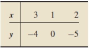
ŷ = 1 - 2x
Expert Solution & Answer
Want to see the full answer?
Check out a sample textbook solution
Students have asked these similar questions
Regression and Predictions. Exercises 13–28 use the same data sets as Exercises 13–28 in Section 10-1. In each case, find the regression equation, letting the first variable be the predictor (x) variable. Find the indicated predicted value by following the prediction procedure summarized in Figure 10-5 on page 493.
Old Faithful Using the listed duration and interval after times, find the best predicted “interval after” time for an eruption with a duration of 253 seconds. How does it compare to an actual eruption with a duration of 253 seconds and an interval after time of 83 minutes?
Regression and Predictions. Exercises 13–28 use the same data sets as Exercises 13–28 in Section 10-1. In each case, find the regression equation, letting the first variable be the predictor (x) variable. Find the indicated predicted value by following the prediction procedure summarized in Figure 10-5 on page 493.
Manatees Use the listed boat/manatee data. In a year not included in the data below, there were 970,000 registered pleasure boats in Florida. Find the best predicted number of manatee fatalities resulting from encounters with boats. Is the result reasonably close to 79, which was the actual number of manatee fatalities?
Using the data in Table 6–11, calculate a 3-month moving average forecast for month 12.
Chapter 14 Solutions
Introductory Statistics (10th Edition)
Ch. 14.1 - Regarding linear equations with one independent...Ch. 14.1 - Prob. 2ECh. 14.1 - Consider the linear equation y = b0 + b1x. a....Ch. 14.1 - Prob. 4ECh. 14.1 - In Exercises 14.514.14, we give linear equations....Ch. 14.1 - Prob. 6ECh. 14.1 - In Exercises 14.5-14.14, we give linear equations....Ch. 14.1 - Prob. 8ECh. 14.1 - Prob. 9ECh. 14.1 - In Exercises 14.514.14, we give linear equations....
Ch. 14.1 - Prob. 11ECh. 14.1 - Prob. 12ECh. 14.1 - Prob. 13ECh. 14.1 - Prob. 14ECh. 14.1 - In Exercises 14.1514.22,we identify the...Ch. 14.1 - Prob. 16ECh. 14.1 - Prob. 17ECh. 14.1 - Prob. 18ECh. 14.1 - Prob. 19ECh. 14.1 - Prob. 20ECh. 14.1 - Prob. 21ECh. 14.1 - Prob. 22ECh. 14.1 - Rental-Car Costs. During one month, the Avis...Ch. 14.1 - Air-Conditioning Repairs. Richards Healing and...Ch. 14.1 - Measuring Temperature. The two most commonly used...Ch. 14.1 - A Law of Physics. A ball is thrown straight up in...Ch. 14.1 - Prob. 27ECh. 14.1 - Prob. 28ECh. 14.1 - Prob. 29ECh. 14.1 - Prob. 30ECh. 14.1 - Prob. 31ECh. 14.1 - Road Grade. The grade of a road is defined as the...Ch. 14.1 - Vertical Lines. In this section, we stated that...Ch. 14.2 - Regarding a scatterplot, a. identify one of its...Ch. 14.2 - Regarding the criterion used to decide on the line...Ch. 14.2 - Regarding the line that best fits a set of data...Ch. 14.2 - Regarding the two variables under consideration in...Ch. 14.2 - Using the regression equation to make predictions...Ch. 14.2 - Fill in the blanks. a. In the context of...Ch. 14.2 - For which of the following sets of data points can...Ch. 14.2 - For which of the following sets of data points can...Ch. 14.2 - In each of Exercises 14.4214.45, we have presented...Ch. 14.2 - In each of Exercises 14.4214.45, we have presented...Ch. 14.2 - In each of Exercises 14.4214.45, we have presented...Ch. 14.2 - In each of Exercises 14.4214.45, we have presented...Ch. 14.2 - For a data set consisting of two data points: a....Ch. 14.2 - Prob. 47ECh. 14.2 - In each of Exercises 14.4814.57, a. find the...Ch. 14.2 - In each of Exercises 14.4814.57. a. find the...Ch. 14.2 - In each of Exercises 14.4814.57, a. find the...Ch. 14.2 - In each of Exercises 14.48-14.57, a. find the...Ch. 14.2 - In each of Exercises 14.4814.57, a. find the...Ch. 14.2 - In each of Exercises 14.4814.57, a. find the...Ch. 14.2 - In each of Exercises 14.48-14.57, a. find the...Ch. 14.2 - In each of Exercises 14.4814.57. a. find the...Ch. 14.2 - In each of Exercises 14.4814.57. a. find the...Ch. 14.2 - In each of Exercises 14.4814.57. a. find the...Ch. 14.2 - Prob. 58ECh. 14.2 - In each of Exercises 14.5814.63, a. find the...Ch. 14.2 - In each of Exercises 14.5814.63. a. find the...Ch. 14.2 - In each of Exercises 14.5814.63, a. find the...Ch. 14.2 - In each of Exercises 14.5814.63. a. find the...Ch. 14.2 - In each of Exercises 14.5814.63, a. find the...Ch. 14.2 - Tax Efficiency. In Exercise 14.58, you determined...Ch. 14.2 - Corvette Prices. In Exercise 14.59, you determined...Ch. 14.2 - Anscombes Quartet. In the article Graphs in...Ch. 14.2 - Study Time and Score. The negative relation...Ch. 14.2 - Age and Price of Orions. In Table 14.2, we...Ch. 14.2 - Wasp Mating Systems. In the paper "Mating System...Ch. 14.2 - In Exercises 14.7014.80, use the technology of...Ch. 14.2 - In Exercises 14.7014.80, use the technology of...Ch. 14.2 - In Exercises 14.7014.80, use the technology of...Ch. 14.2 - In Exercises I4.7014.80, use the technology of...Ch. 14.2 - In Exercises 14.7014.80, use the technology of...Ch. 14.2 - In Exercises 14.7014.80, use the technology of...Ch. 14.2 - Prob. 76ECh. 14.2 - Prob. 77ECh. 14.2 - Prob. 78ECh. 14.2 - Prob. 79ECh. 14.2 - In Exercises 14.7014.80, use the technology of...Ch. 14.2 - Prob. 81ECh. 14.2 - Time Series. A collection of observations of a...Ch. 14.3 - In this section, we introduced a descriptive...Ch. 14.3 - A measure of total variation in the observed...Ch. 14.3 - A measure of the amount of variation in the...Ch. 14.3 - A measure of the amount of variation in the...Ch. 14.3 - Prob. 87ECh. 14.3 - In Exercises 14.8814.97, we repeal the data and...Ch. 14.3 - In Exercises14.481497, we repeal the tiara and...Ch. 14.3 - In Exercises 14.8814.97, we repeat the data and...Ch. 14.3 - Prob. 91ECh. 14.3 - Prob. 92ECh. 14.3 - Prob. 93ECh. 14.3 - Prob. 94ECh. 14.3 - Prob. 95ECh. 14.3 - Prob. 96ECh. 14.3 - Prob. 97ECh. 14.3 - Applying the Concepts and Skills For Exercises...Ch. 14.3 - Prob. 99ECh. 14.3 - Prob. 100ECh. 14.3 - Prob. 101ECh. 14.3 - Prob. 102ECh. 14.3 - For Exercises 14.9814.103, a. compute SST, SSR,...Ch. 14.3 - Prob. 104ECh. 14.3 - In Exercises 14.10414.115, use the technology of...Ch. 14.3 - Prob. 106ECh. 14.3 - Prob. 107ECh. 14.3 - Prob. 108ECh. 14.3 - Prob. 109ECh. 14.3 - Prob. 110ECh. 14.3 - Prob. 111ECh. 14.3 - Prob. 112ECh. 14.3 - Prob. 113ECh. 14.3 - In Exercises 14.10414.115, use the technology of...Ch. 14.3 - In Exercises 14.10414.115, use the technology of...Ch. 14.3 - What can you say about SSE, SSR, and the utility...Ch. 14.3 - As we noted, because of the regression identity,...Ch. 14.4 - What is one purpose of the linear correlation...Ch. 14.4 - Prob. 119ECh. 14.4 - The symbol that is used for the linear correlation...Ch. 14.4 - A value of r close to 1 indicates that there is a...Ch. 14.4 - A value of r close to ____ indicates that there is...Ch. 14.4 - A value of r close to ____ indicates that the...Ch. 14.4 - A value of r close to 0 indicates that the...Ch. 14.4 - If y tends to increase linearly as x increases,...Ch. 14.4 - If y lends to decrease linearly as x increases,...Ch. 14.4 - If there is no linear relationship between x and...Ch. 14.4 - In each of Exercises 14.12814.130, determine...Ch. 14.4 - In each of Exercises 14.12814.130, determine...Ch. 14.4 - In each of Exercises 14.12814.130, determine...Ch. 14.4 - Answer true or false to the following statement...Ch. 14.4 - The linear correlation coefficient of a set of...Ch. 14.4 - The coefficient of determination of a set of data...Ch. 14.4 - In Exercises 14.13414.143, we repeat data from...Ch. 14.4 - In Exercises 14.13414.143, we repeat data from...Ch. 14.4 - In Exercises 14.13414.143, we repeat data front...Ch. 14.4 - Prob. 137ECh. 14.4 - In Exercises 14.13414.143, we repeat data from...Ch. 14.4 - In Exercises 14.13414.143, we repeat data from...Ch. 14.4 - In Exercises 14.13414.143, we repeat data from...Ch. 14.4 - In Exercises 14.13414.143, we repeat data from...Ch. 14.4 - In Exercises 14.13414.143, we repeat data from...Ch. 14.4 - In Exercises 14.13414.143, we repeat data from...Ch. 14.4 - In Exercises 14.14414.149, we repeat data from...Ch. 14.4 - In Exercises 14.14414.149, we repeat data from...Ch. 14.4 - In Exercises 14.14414.149, we repeat data from...Ch. 14.4 - Prob. 147ECh. 14.4 - In Exercises 14.14414.149, we repeat data from...Ch. 14.4 - In Exercises 14.14414.149, we repeat data from...Ch. 14.4 - Height and Score. A random sample of 10 students...Ch. 14.4 - Prob. 151ECh. 14.4 - Prob. 152ECh. 14.4 - Prob. 153ECh. 14.4 - Prob. 154ECh. 14.4 - In Exercise 14.154-14.166, use the technology of...Ch. 14.4 - Prob. 156ECh. 14.4 - Prob. 157ECh. 14.4 - Prob. 158ECh. 14.4 - Prob. 159ECh. 14.4 - Prob. 160ECh. 14.4 - Prob. 161ECh. 14.4 - In Exercises 14.154-14.166, use the technology of...Ch. 14.4 - In Exercises 14.15414.166, use the technology of...Ch. 14.4 - Prob. 164ECh. 14.4 - Prob. 165ECh. 14.4 - In Exercises 14.154-14.166, use the technology of...Ch. 14.4 - The coefficient of determination of a set of data...Ch. 14.4 - Country Music Blues. A Knight-Ridder News Service...Ch. 14.4 - Prob. 169ECh. 14.4 - In each of Exercises 14.169 and 14.170, a....Ch. 14 - For a linear equation y = b0 + b1x, identify the ...Ch. 14 - Consider the linear equation y = 4-3x. a. At what...Ch. 14 - In Problems 35, answer true or false to each...Ch. 14 - In Problems 35, answer true or false to each...Ch. 14 - In Problems 35, answer true or false to each...Ch. 14 - Prob. 6RPCh. 14 - In Problems 35, answer true or false to each...Ch. 14 - Prob. 8RPCh. 14 - In each of Problems 911, fill in the blank. 9....Ch. 14 - Prob. 10RPCh. 14 - Prob. 11RPCh. 14 - Prob. 12RPCh. 14 - Prob. 13RPCh. 14 - Prob. 14RPCh. 14 - Prob. 15RPCh. 14 - Prob. 16RPCh. 14 - Prob. 17RPCh. 14 - Prob. 18RPCh. 14 - Prob. 19RPCh. 14 - Equipment Depreciation. A small company has...Ch. 14 - Graduation Rates. Graduation ratethe percentage of...Ch. 14 - Graduation Rates. Refer to Problem 21. a....Ch. 14 - Graduation Rates. Refer to Problem 21. a. Compute...Ch. 14 - Exotic Plants. In the article Effects of Human...Ch. 14 - In Problems 2527, use the technology of your...Ch. 14 - Prob. 26RPCh. 14 - Prob. 27RPCh. 14 - Recall from Chapter 1 (see page 34) that the Focus...Ch. 14 - At the beginning of this chapter, we presented...
Knowledge Booster


Learn more about
Need a deep-dive on the concept behind this application? Look no further. Learn more about this topic, statistics and related others by exploring similar questions and additional content below.Similar questions
- A researcher believes that the so-called “sugar high” is not real. He gathered 30 adolescents and recorded their activity level in the scale of 0 – 100 (0 = not active and 100 = super active). First, he recorded participants’ activity level before they consumed candy. After recording their pre-sugar activity level, the researcher gave out 5 Snickers bars to participants. Then, he recorded their post-sugar activity level. The average difference between post-sugar and pre-sugar activity level is 50 (i.e., the activity levels are higher after sugar than prior to it) with a standard deviation of 10. A). Complete test statistic and critical values B). Conclusionarrow_forwardA researcher believes that the so-called “sugar high” is not real. He gathered 30 adolescents and recorded their activity level in the scale of 0 – 100 (0 = not active and 100 = super active). First, he recorded participants’ activity level before they consumed candy. After recording their pre-sugar activity level, the researcher gave out 5 Snickers bars to participants. Then, he recorded their post-sugar activity level. The average difference between post-sugar and pre-sugar activity level is 50 (i.e., the activity levels are higher after sugar than prior to it) with a standard deviation of 10. A). What is the type of test you will use? (z-test, single-sample t-test, paired-samples t-test, or independent samples t-test) and why (what information provided in the problem)B). What are the hypotheses (Be Specific)arrow_forwarda.State the predictors available in this model.arrow_forward
- Using the data in Table 6–11, calculate a 3-month moving average forecastfor month 12.arrow_forwardWhich model—the one for parliaments or the one for ministries (or cabinets)—presented in the article has the greater explanatory power? How can you tell?arrow_forward2.62 For the period 2001–2008, the Bristol-Myers Squibb Company, Inc. reported the following amounts (in billions of dollars) for (1) net sales and (2) advertising and product promotion. The data are also in the file XR02062. Source: Bristol-Myers Squibb Company, Annual Reports, 2005, 2008. Year Net Sales Advertising/Promotion 2001 $16.612 $1.201 2002 16.208 1.143 2003 18.653 1.416 2004 19.380 1.411 2005 19.207 1.476 2006 16.208 1.304 2007 18.193 1.415 2008 20.597 1.550 For these data, construct a line graph that shows both net sales and expenditures for advertising/product promotion over time. Some would suggest that increases in advertising should be accompanied by increases in sales. Does your line graph support this?arrow_forward
- The body mass index (BMI) of a person is the person’s weight divided by the square of his or her height. It is an indirect measure of the person’s body fat and an indicator of obesity. Results from surveys conducted by the Centers for Disease Control and Prevention (CDC) showed that the estimated mean BMI for US adults increased from 25.0 in the 1960–1962 period to 28.1 in the 1999–2002 period. [Source: Ogden, C., et al. (2004). Mean body weight, height, and body mass index, United States 1960–2002. Suppose you are a health researcher. You conduct a hypothesis test to determine whether the mean BMI of US adults in the current year is greater than the mean BMI of US adults in 2000. Assume that the mean BMI of US adults in 2000 was 28.1 (the population mean). You obtain a sample of BMI measurements of 1,034 US adults, which yields a sample mean of M = 28.9. Let μ denote the mean BMI of US adults in the current year. Please Formulate the null and alternative hypothesesarrow_forwardQ1. The table provided gives data on indexes of output per hour (X) and real compensation per hour (Y) for the business and nonfarm business sectors of the U.S. economy for 1960–2005. The base year of the indexes is 1992 = 100 and the indexes are seasonally adjusted. a. Plot Y against X for the two sectors separately. b. What is the economic theory behind the relationship between the two variables? Does the scattergram support the theory? c. Estimate the OLS regression of Y on X. Note: on the table ( 1. Output refers to real gross domestic product in the sector. 2. Wages and salaries of employees plus employers’ contributions for social insurance and private benefit plans. 3. Hourly compensation divided by the consumer price index for all urban consumers for recent quarters.) Thank you!arrow_forwardLarge companies typically collect volumes of data before designing a product, not only to gain information as to whether the product should be released, but also to pinpoint which markets would be the best targets for the product. Several months ago, I was interviewed by such a company while shopping at a mall. I was asked about my exercise habits and whether or not I'd be interested in buying a video/DVD designed to teach stretching exercises. I fall into the male, 18 – 35-years-old category, and I guessed that, like me, many males in that category would not be interested in a stretching video. My friend Amanda falls in the female, older-than-35 category, and I was thinking that she might like the stretching video. After being interviewed, I looked at the interviewer's results. Of the 97 people in my market category who had been interviewed, 16 said they would buy the product, and of the 101 people in Amanda's market category, 31 said they would buy it. Assuming that these data came…arrow_forward
- Large companies typically collect volumes of data before designing a product, not only to gain information as to whether the product should be released, but also to pinpoint which markets would be the best targets for the product. Several months ago, I was interviewed by such a company while shopping at a mall. I was asked about my exercise habits and whether or not I'd be interested in buying a video/DVD designed to teach stretching exercises. I fall into the male, 18 – 35-years-old category, and I guessed that, like me, many males in that category would not be interested in a stretching video. My friend Diane falls in the female, older-than-35 category, and I was thinking that she might like the stretching video. After being interviewed, I looked at the interviewer's results. Of the 93 people in my market category who had been interviewed, 17 said they would buy the product, and of the 113 people in Diane's market category, 34 said they would buy it. Assuming that these data came…arrow_forwardHeart rate during laughter. Laughter is often called “the best medicine,” since studies have shown that laughter can reduce muscle tension and increase oxygenation of the blood. In the International Journal of Obesity (Jan. 2007), researchers at Vanderbilt University investigated the physiological changes that accompany laughter. Ninety subjects (18–34 years old) watched film clips designed to evoke laughter. During the laughing period, the researchers measured the heart rate (beats per minute) of each subject, with the following summary results: Mean = 73.5, Standard Deviation = 6. n=90 (we can treat this as a large sample and use z) It is well known that the mean resting heart rate of adults is 71 beats per minute. Based on the research on laughter and heart rate, we would expect subjects to have a higher heart beat rate while laughing.Construct 95% Confidence interval using z value. What is the lower bound of CI? a) Calculate the value of the test statistic.(z*) b) If…arrow_forwardBecause of high tuition costs at state and private universities, enrollments atcommunity colleges have increased dramatically in recent years. The following data show theenrollment (in thousands) for Jefferson Community College from 2001–2009:Year Period (t) Enrollment (1000s)2001 1 6.52002 2 8.12003 3 8.42004 4 10.22005 5 12.52006 6 13.32007 7 13.72008 8 17.22009 9 18.1Compute F10: the Forecast for 2010. Compute Pearson’s Correlation Coefficient Use the Method of Least Squares to obtain the Best-Fit-Line for this data. Use the line to compute the forecast.arrow_forward
arrow_back_ios
SEE MORE QUESTIONS
arrow_forward_ios
Recommended textbooks for you
 MATLAB: An Introduction with ApplicationsStatisticsISBN:9781119256830Author:Amos GilatPublisher:John Wiley & Sons Inc
 Probability and Statistics for Engineering and th...StatisticsISBN:9781305251809Author:Jay L. DevorePublisher:Cengage Learning
 Statistics for The Behavioral Sciences (MindTap C...StatisticsISBN:9781305504912Author:Frederick J Gravetter, Larry B. WallnauPublisher:Cengage Learning
 Elementary Statistics: Picturing the World (7th E...StatisticsISBN:9780134683416Author:Ron Larson, Betsy FarberPublisher:PEARSON
 The Basic Practice of StatisticsStatisticsISBN:9781319042578Author:David S. Moore, William I. Notz, Michael A. FlignerPublisher:W. H. Freeman
 Introduction to the Practice of StatisticsStatisticsISBN:9781319013387Author:David S. Moore, George P. McCabe, Bruce A. CraigPublisher:W. H. Freeman
MATLAB: An Introduction with Applications
Statistics
ISBN:9781119256830
Author:Amos Gilat
Publisher:John Wiley & Sons Inc
Probability and Statistics for Engineering and th...
Statistics
ISBN:9781305251809
Author:Jay L. Devore
Publisher:Cengage Learning
Statistics for The Behavioral Sciences (MindTap C...
Statistics
ISBN:9781305504912
Author:Frederick J Gravetter, Larry B. Wallnau
Publisher:Cengage Learning
Elementary Statistics: Picturing the World (7th E...
Statistics
ISBN:9780134683416
Author:Ron Larson, Betsy Farber
Publisher:PEARSON
The Basic Practice of Statistics
Statistics
ISBN:9781319042578
Author:David S. Moore, William I. Notz, Michael A. Fligner
Publisher:W. H. Freeman
Introduction to the Practice of Statistics
Statistics
ISBN:9781319013387
Author:David S. Moore, George P. McCabe, Bruce A. Craig
Publisher:W. H. Freeman
Correlation Vs Regression: Difference Between them with definition & Comparison Chart; Author: Key Differences;https://www.youtube.com/watch?v=Ou2QGSJVd0U;License: Standard YouTube License, CC-BY
Correlation and Regression: Concepts with Illustrative examples; Author: LEARN & APPLY : Lean and Six Sigma;https://www.youtube.com/watch?v=xTpHD5WLuoA;License: Standard YouTube License, CC-BY